Upward derivative of a regular grid

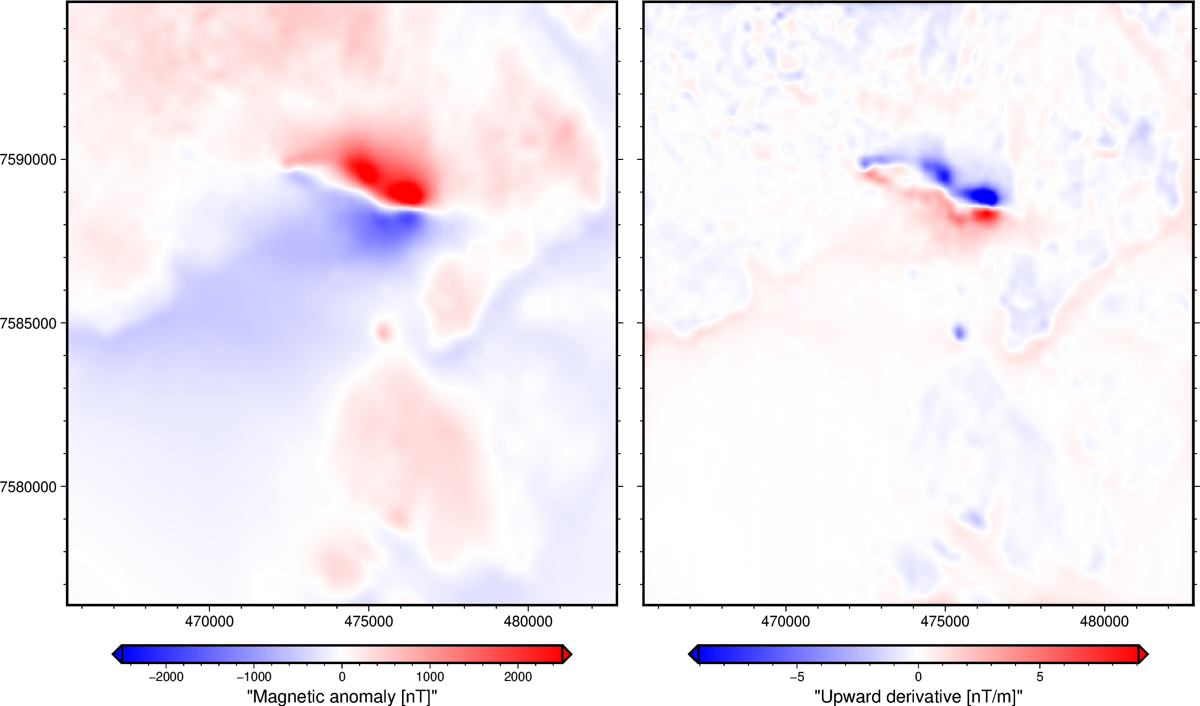
Upward derivative:
 <xarray.DataArray (northing: 370, easting: 346)> Size: 1MB
array([[ 0.00392149, -0.03020041, -0.03536756, ..., -0.04226171,
        -0.04011395, -0.05324249],
       [-0.03893551, -0.06934878, -0.06971427, ..., -0.02488467,
        -0.02337474, -0.03747796],
       [-0.04212395, -0.07421057, -0.07659479, ..., -0.02333065,
        -0.02383248, -0.03317766],
       ...,
       [-0.24893064, -0.07536529,  0.02301565, ...,  0.17154972,
         0.32659791,  0.52662516],
       [-0.25872989, -0.10818937, -0.00694061, ...,  0.16703944,
         0.3530013 ,  0.5823102 ],
       [-0.15762632, -0.04329555,  0.02397919, ...,  0.08397172,
         0.23195226,  0.4514189 ]], shape=(370, 346))
Coordinates:
  * northing  (northing) float64 3kB 7.576e+06 7.576e+06 ... 7.595e+06 7.595e+06
  * easting   (easting) float64 3kB 4.655e+05 4.656e+05 ... 4.827e+05 4.828e+05
    height    (northing, easting) float64 1MB 500.0 500.0 500.0 ... 500.0 500.0

import ensaio
import pygmt
import verde as vd
import xarray as xr

import harmonica as hm

# Fetch magnetic grid over the Lightning Creek Sill Complex, Australia using
# Ensaio and load it with Xarray
fname = ensaio.fetch_lightning_creek_magnetic(version=1)
magnetic_grid = xr.load_dataarray(fname)

# Compute the upward derivative of the grid
deriv_upward = hm.derivative_upward(magnetic_grid)
# Show the upward derivative
print("\nUpward derivative:\n", deriv_upward)


# Plot original magnetic anomaly and the upward derivative
fig = pygmt.Figure()
with fig.subplot(nrows=1, ncols=2, figsize=("28c", "15c"), sharey="l"):
    with fig.set_panel(panel=0):
        # Make colormap of data
        scale = 2500
        pygmt.makecpt(cmap="polar+h", series=[-scale, scale], background=True)
        # Plot magnetic anomaly grid
        fig.grdimage(
            grid=magnetic_grid,
            projection="X?",
            cmap=True,
        )
        # Add colorbar
        fig.colorbar(
            frame='af+l"Magnetic anomaly [nT]"',
            position="JBC+h+o0/1c+e",
        )
    with fig.set_panel(panel=1):
        # Make colormap for upward derivative (saturate it a little bit)
        scale = 0.6 * vd.maxabs(deriv_upward)
        pygmt.makecpt(cmap="polar+h", series=[-scale, scale], background=True)
        # Plot upward derivative
        fig.grdimage(grid=deriv_upward, projection="X?", cmap=True)
        # Add colorbar
        fig.colorbar(
            frame='af+l"Upward derivative [nT/m]"',
            position="JBC+h+o0/1c+e",
        )
fig.show()