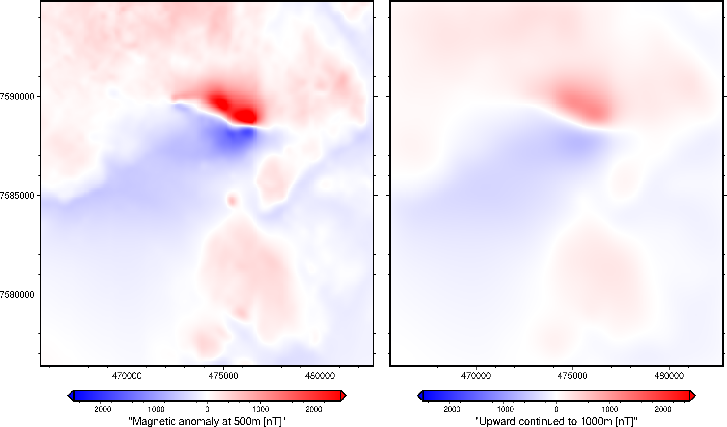
Upward continuation of a regular grid

Upward continued magnetic grid:
 <xarray.DataArray (northing: 370, easting: 346)> Size: 1MB
array([[  19.55620825,   19.27947097,   18.97006949, ..., -104.5277715 ,
        -104.00305377, -103.51237675],
       [  19.11131778,   18.83284215,   18.52168951, ..., -104.97064033,
        -104.450267  , -103.96352053],
       [  18.63232495,   18.35205701,   18.03910509, ..., -105.44585262,
        -104.93001717, -104.44733358],
       ...,
       [ 161.38902102,  161.11651289,  160.87879242, ...,    0.45282316,
          -3.73975786,   -7.71323984],
       [ 160.97996734,  160.69101224,  160.43830842, ...,    3.41228276,
          -0.93864591,   -5.06866624],
       [ 160.59789277,  160.29497591,  160.02940435, ...,    6.13383277,
           1.64184139,   -2.62848316]], shape=(370, 346))
Coordinates:
  * northing  (northing) float64 3kB 7.576e+06 7.576e+06 ... 7.595e+06 7.595e+06
  * easting   (easting) float64 3kB 4.655e+05 4.656e+05 ... 4.827e+05 4.828e+05

import ensaio
import pygmt
import xarray as xr

import harmonica as hm

# Fetch magnetic grid over the Lightning Creek Sill Complex, Australia using
# Ensaio and load it with Xarray
fname = ensaio.fetch_lightning_creek_magnetic(version=1)
magnetic_grid = xr.load_dataarray(fname)

# Upward continue the magnetic grid, from 500 m to 1000 m
# (a height displacement of 500m)
upward_continued = hm.upward_continuation(magnetic_grid, height_displacement=500)
# Show the upward continued grid
print("\nUpward continued magnetic grid:\n", upward_continued)


# Plot original magnetic anomaly and the upward continued grid
fig = pygmt.Figure()
with fig.subplot(nrows=1, ncols=2, figsize=("28c", "15c"), sharey="l"):
    # Make colormap for both plots data
    scale = 2500
    pygmt.makecpt(cmap="polar+h", series=[-scale, scale], background=True)
    with fig.set_panel(panel=0):
        # Plot magnetic anomaly grid
        fig.grdimage(
            grid=magnetic_grid,
            projection="X?",
            cmap=True,
        )
        # Add colorbar
        fig.colorbar(
            frame='af+l"Magnetic anomaly at 500m [nT]"',
            position="JBC+h+o0/1c+e",
        )
    with fig.set_panel(panel=1):
        # Plot upward continued grid
        fig.grdimage(grid=upward_continued, projection="X?", cmap=True)
        # Add colorbar
        fig.colorbar(
            frame='af+l"Upward continued to 1000m [nT]"',
            position="JBC+h+o0/1c+e",
        )
fig.show()