Rectangular prisms#
One of the geometric bodies that Harmonica is able to forward model are
rectangular prisms.
We can compute their gravitational fields through the
harmonica.prism_gravity function.
Rectangular prisms can only be defined in Cartesian coordinates, therefore they are intended to be used to forward model bodies in a small geographic region, in which we can neglect the curvature of the Earth.
Each prism can be defined as a tuple containing its boundaries in the following order: west, east, south, north, bottom, top in Cartesian coordinates and in meters.
Let’s define a single prism and compute the gravitational potential it generates on a computation point located at 500 meters above its uppermost surface.
Define the prism and its density (in kg per cubic meters):
prism = (-100, 100, -100, 100, -1000, 500)
density = 3000
Define a computation point located 500 meters above the top surface of the prism:
coordinates = (0, 0, 1000)
And finally, compute the gravitational potential field it generates on the computation point:
potential = hm.prism_gravity(coordinates, prism, density, field="potential")
print(potential, "J/kg")
0.011053722963867401 J/kg
Gravitational fields#
The harmonica.prism_gravity is able to compute the gravitational
potential ("potential"), the acceleration components ("g_e", "g_n",
"g_z"), and tensor components ("g_ee", "g_nn", "g_zz",
"g_en", "g_ez", "g_nz").
Build a regular grid of computation points located 10m above the zero height:
import bordado as bd

region = (-10e3, 10e3, -10e3, 10e3)
shape = (51, 51)
height = 10
coordinates = bd.grid_coordinates(
    region, shape=shape, non_dimensional_coords=height
)
Define a single prism:
prism = [-2e3, 2e3, -2e3, 2e3, -1.6e3, -900]
density = 3300
Compute the gravitational fields that this prism generate on each observation point:
fields = (
   "potential",
   "g_e", "g_n", "g_z",
   "g_ee", "g_nn", "g_zz", "g_en", "g_ez", "g_nz"
)

results = {}
for field in fields:
   results[field] = hm.prism_gravity(coordinates, prism, density, field=field)
We can reshape the results into variables of an dataset:
import verde as vd

grid = vd.make_xarray_grid(
   coordinates,
   tuple(results.values()),
   data_names=results.keys(),
   extra_coords_names="extra",
)
grid
<xarray.Dataset> Size: 230kB
Dimensions:    (northing: 51, easting: 51)
Coordinates:
  * northing   (northing) float64 408B -1e+04 -9.6e+03 ... 9.6e+03 1e+04
  * easting    (easting) float64 408B -1e+04 -9.6e+03 -9.2e+03 ... 9.6e+03 1e+04
    extra      (northing, easting) float64 21kB 10.0 10.0 10.0 ... 10.0 10.0
Data variables:
    potential  (northing, easting) float64 21kB 0.1743 0.1778 ... 0.1778 0.1743
    g_e        (northing, easting) float64 21kB 0.8702 0.8869 ... -0.8702
    g_n        (northing, easting) float64 21kB 0.8702 0.9239 ... -0.8702
    g_z        (northing, easting) float64 21kB 0.1118 0.1188 ... 0.1188 0.1118
    g_ee       (northing, easting) float64 21kB 0.4327 0.4027 ... 0.4027 0.4327
    g_nn       (northing, easting) float64 21kB 0.4327 0.5159 ... 0.5159 0.4327
    g_zz       (northing, easting) float64 21kB -0.8654 -0.9186 ... -0.8654
    g_en       (northing, easting) float64 21kB 1.304 1.383 ... 1.383 1.304
    g_ez       (northing, easting) float64 21kB 0.1697 0.1803 ... -0.1697
g_nz (northing, easting) float64 21kB 0.1697 0.1878 ... -0.1697Plot the results:
import matplotlib.pyplot as plt

grid.potential.plot(cbar_kwargs={"label":"J/kg"})
plt.gca().set_aspect("equal")
plt.show()
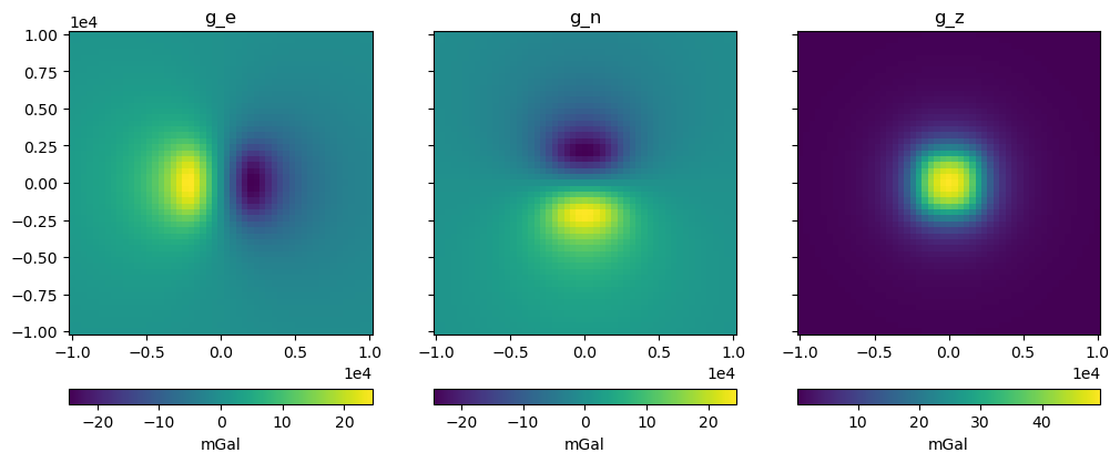
fig, axes = plt.subplots(nrows=1, ncols=3, sharey=True, figsize=(12, 8))

fields = ["g_e", "g_n", "g_z"]
maxabs = vd.maxabs(*[grid[f] for f in fields], percentile=99)
for field, ax in zip(fields, axes):
   tmp = grid[field].plot(
      ax=ax,
      add_colorbar=False,
      vmin=-maxabs,
      vmax=maxabs,
      cmap='RdBu_r',
   )
   ax.set_aspect("equal")
   ax.set_title(field)
fig.colorbar(tmp, ax=axes.ravel().tolist(), orientation="horizontal", label="mGal", fraction=.03, pad=0.08)
plt.show()
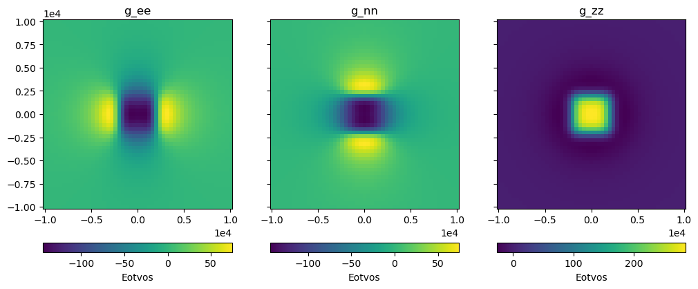
fig, axes = plt.subplots(nrows=1, ncols=3, sharey=True, figsize=(12, 8))

fields = ["g_ee", "g_nn", "g_zz"]
maxabs = vd.maxabs(*[grid[f] for f in fields], percentile=99)
for field, ax in zip(fields, axes):
   tmp = grid[field].plot(
      ax=ax,
      add_colorbar=False,
      vmin=-maxabs,
      vmax=maxabs,
      cmap='RdBu_r',
   )
   ax.set_aspect("equal")
   ax.set_title(field)
fig.colorbar(tmp, ax=axes.ravel().tolist(), orientation="horizontal", label="Eotvos", fraction=.03, pad=0.08)
plt.show()
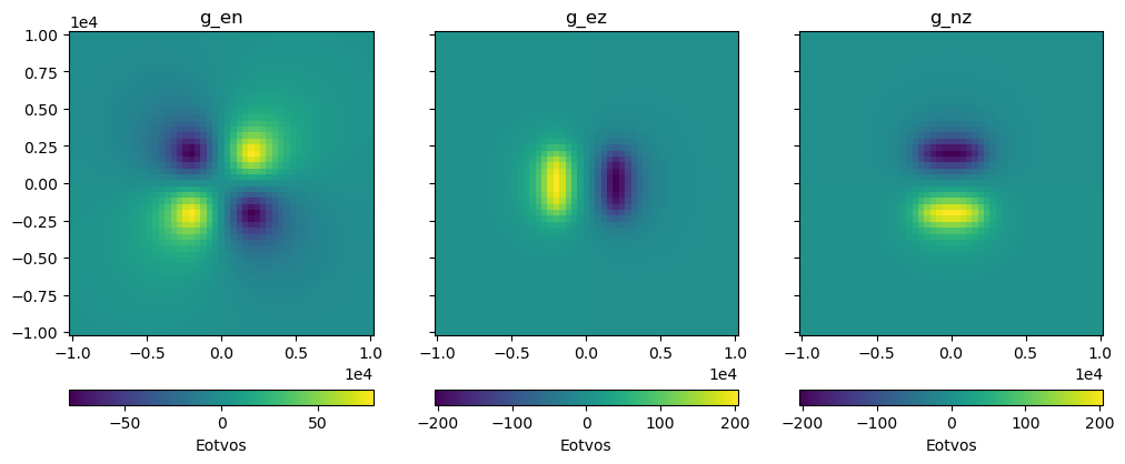
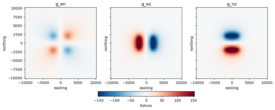
fig, axes = plt.subplots(nrows=1, ncols=3, sharey=True, figsize=(12, 8))

fields = ["g_en", "g_ez", "g_nz"]
maxabs = vd.maxabs(*[grid[f] for f in fields], percentile=99)
for field, ax in zip(fields, axes):
   tmp = grid[field].plot(
      ax=ax,
      add_colorbar=False,
      vmin=-maxabs,
      vmax=maxabs,
      cmap='RdBu_r',
   )
   ax.set_aspect("equal")
   ax.set_title(field)
fig.colorbar(tmp, ax=axes.ravel().tolist(), orientation="horizontal", label="Eotvos", fraction=.03, pad=0.08)
plt.show()
Passing multiple prisms#
We can compute the gravitational field of a set of prisms by passing a list of
them, where each prism is defined as mentioned before, and then making
a single call of the harmonica.prism_gravity function.
Lets define a set of four prisms, along with their densities:
prisms = [
    [2e3, 3e3, 2e3, 3e3, -10e3, -1e3],
    [3e3, 4e3, 7e3, 8e3, -9e3, -1e3],
    [7e3, 8e3, 1e3, 2e3, -7e3, -1e3],
    [8e3, 9e3, 6e3, 7e3, -8e3, -1e3],
]
densities = [2670, 3300, 2900, 2980]
We can define a set of computation points located on a regular grid at zero height:
import bordado as bd

coordinates = bd.grid_coordinates(
    region=(0, 10e3, 0, 10e3), shape=(40, 40), non_dimensional_coords=0
)
And finally calculate the vertical component of the gravitational acceleration generated by the whole set of prisms on every computation point:
g_z = hm.prism_gravity(coordinates, prisms, densities, field="g_z")
Note
When passing multiple prisms and coordinates to
harmonica.prism_gravity we calculate the field in parallel using
multiple CPUs, speeding up the computation.
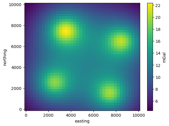
Lets plot this gravitational field:
grid = vd.make_xarray_grid(
   coordinates, g_z, data_names="g_z", extra_coords_names="extra")
grid.g_z.plot(cbar_kwargs={"label":"mGal"})
<matplotlib.collections.QuadMesh at 0x7f4a861ed670>
Magnetic fields#
The harmonica.prism_magnetic function allows us to calculate the
magnetic fields generated by rectangular prisms on a set of observation points.
Each rectangular prism is defined in the same way we did for the gravity
forward modelling, although we now need to define a magnetization vector for
each one of them.
For example:
import numpy as np

prisms = [
    [-5e3, -3e3, -5e3, -2e3, -10e3, -1e3],
    [3e3, 4e3, 4e3, 5e3, -9e3, -1e3],
]

magnetization_easting = np.array([0.5, -0.4])
magnetization_northing = np.array([0.5, 0.3])
magnetization_upward = np.array([-0.78989, 0.2])
magnetization = (
   magnetization_easting, magnetization_northing, magnetization_upward
)
The magnetization should be a tuple of three arrays: the easting, northing
and upward components of the magnetization vector (in \(Am^{-1}\)) for each
prism in prisms.
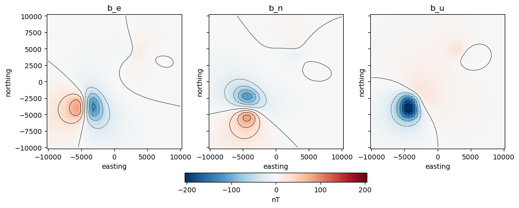
We can use the harmonica.prism_magnetic function to compute the three
components of the magnetic field the prisms generate on any set of observation
points by choosing field="b":
region = (-10e3, 10e3, -10e3, 10e3)
shape = (51, 51)
height = 10
coordinates = bd.grid_coordinates(
    region, shape=shape, non_dimensional_coords=height
)
b_e, b_n, b_u = hm.prism_magnetic(coordinates, prisms, magnetization, field="b")
We can reshape the results into variables of an dataset:
grid = vd.make_xarray_grid(
   coordinates,
   data=(b_e, b_n, b_u),
   data_names=["b_e", "b_n", "b_u"],
   extra_coords_names="extra"
)
fig, axes = plt.subplots(nrows=1, ncols=3, sharey=True, figsize=(12, 8))

maxabs = vd.maxabs(*[grid[v] for v in grid.variables], percentile=99)
for field, ax in zip(grid.variables, axes):
   tmp = grid[field].plot(
      ax=ax,
      add_colorbar=False,
      vmin=-maxabs,
      vmax=maxabs,
      cmap='RdBu_r',
   )
   grid[field].plot.contour(
      ax=ax,
      colors="k",
      linewidths=0.5,
   )
   ax.set_aspect("equal")
   ax.set_title(field)
fig.colorbar(tmp, ax=axes.ravel().tolist(), orientation="horizontal", label="nT", fraction=.03, pad=0.08)
plt.show()
Alternatively, we can compute just a single component by choosing field to
be:
"b_e"for the easting component,"b_n"for the northing component, and"b_u"for the upward component.
Important
Computing the three components at the same time with field="b" is more
efficient than computing each one of the three components independently.
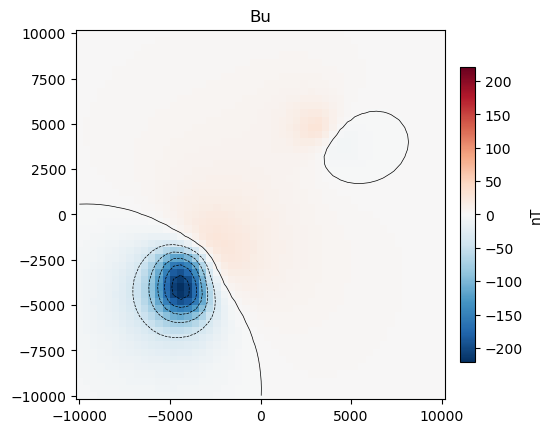
For example, we can calculate only the upward component of the magnetic field generated by these two prisms:
b_u = hm.prism_magnetic(
   coordinates, prisms, magnetization, field="b_u"
)
maxabs = vd.maxabs(b_u)

tmp = plt.pcolormesh(
   coordinates[0], coordinates[1], b_u, vmin=-maxabs, vmax=maxabs, cmap="RdBu_r"
)
plt.contour(coordinates[0], coordinates[1], b_u, colors="k", linewidths=0.5)
plt.title("Bu")
plt.gca().set_aspect("equal")
plt.colorbar(tmp, label="nT", pad=0.03, shrink=0.8)
plt.show()
Prism layer#
One of the most common usage of prisms is to model geologic structures.
Harmonica offers the possibility to define a layer of prisms through the
harmonica.prism_layer function: a regular grid of
prisms of equal size along the horizontal dimensions and with variable top and
bottom boundaries.
It returns a xarray.Dataset with the coordinates of the centers of the
prisms and their corresponding physical properties.
The harmonica.DatasetAccessorPrismLayer Dataset accessor can be used
to obtain some properties of the layer like its shape and size or the
boundaries of any prism in the layer.
Moreover, we can use the harmonica.DatasetAcessorPrismLayer.gravity
method to compute the gravitational field of the prism layer on any set of
computation points.
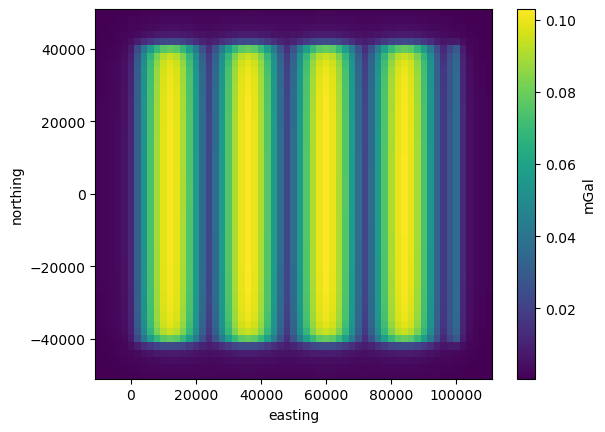
Lets create a simple prism layer, whose lowermost boundaries will be set on zero and their uppermost boundary will approximate a sinusoidal function. We can start by setting the region of the layer and the horizontal dimensions of the prisms:
region = (0, 100e3, -40e3, 40e3)
spacing = 2000
Then we can define a regular grid where the centers of the prisms will fall:
easting, northing = bd.grid_coordinates(region=region, spacing=spacing)
We need to define a 2D array for the uppermost surface of the layer. We will sample a trigonometric function for this simple example:
wavelength = 24 * spacing
surface = np.abs(np.sin(easting * 2 * np.pi / wavelength))
Let’s assign the same density to each prism through a 2d array with the same value: 2700 kg per cubic meter.
density = np.full_like(surface, 2700)
Now we can define the prism layer specifying the reference level to zero:
prisms = hm.prism_layer(
    coordinates=(easting, northing),
    surface=surface,
    reference=0,
    properties={"density": density},
)
Let’s define a grid of observation points at 1 km above the zeroth height:
region_pad = bd.pad_region(region, 10e3)
coordinates = bd.grid_coordinates(
    region_pad, spacing=spacing, non_dimensional_coords=1e3
)
And compute the gravitational field generated by the prism layer on them:
gravity = prisms.prism_layer.gravity(coordinates, field="g_z")
Finally, let’s plot the gravitational field:
grid = vd.make_xarray_grid(
   coordinates, gravity, data_names="gravity", extra_coords_names="extra")

grid.gravity.plot(cbar_kwargs={"label":"mGal"})
<matplotlib.collections.QuadMesh at 0x7f4a8594ffb0>