Point sources#
We can compute the gravitational field of point masses through the
harmonica.point_gravity function.
It offers the possibility to define point sources and computation points either
in Cartesian or in spherical coordinates.
Each point mass can be defined as a tuple containing its coordinates in the following order: easting, northing and upward (in Cartesian coordinates) or longitude, spherical latitude and radius (in spherical coordinates).
Cartesian coordinates#
For example, lets define a single point mass and compute the gravitational potential it generates on a computation point located 100 meters above it.
Define the point source and its mass (in kg):
point = (400, 300, 200)
mass = 1e6
Define a computation point located 100m above the point source:
coordinates = (point[0], point[1], point[2] + 100)
And finally, compute the gravitational potential field it generates on the computation point:
potential = hm.point_gravity(coordinates, point, mass, field="potential")
print(potential, "J/kg")
6.674299999999999e-07 J/kg
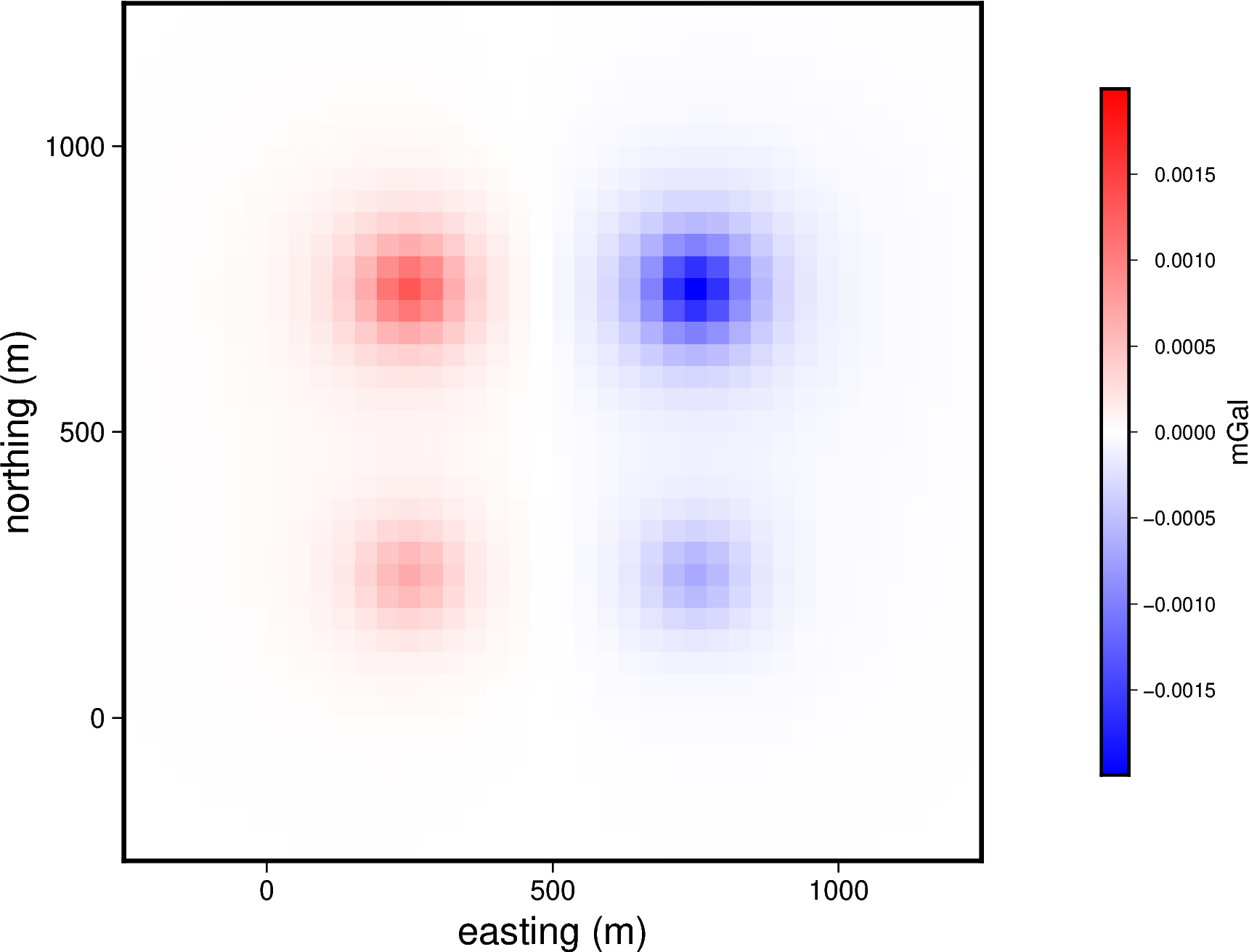
Working with multiple sources#
We can easily compute the gravitational field of a set of point sources by
grouping its coordinates in arrays and with a single call of the
harmonica.point_gravity.
Lets define a set of four point sources, along with their masses:
import numpy as np

easting = np.array([250, 750, 250, 750])
northing = np.array([250, 250, 750, 750])
upward = np.array([-100, -100, -100, -100])
points = (easting, northing, upward)

masses = np.array([1e6, -1e6, 2e6, -3e6])
We can define a set of computation points located on a regular grid at zero height:
import bordado as bd

coordinates = bd.grid_coordinates(
    region=(-250, 1250, -250, 1250), shape=(40, 40), non_dimensional_coords=0
)
And finally calculate the vertical component of the gravitational acceleration generated by the whole set of point sources on every computation point:
g_z = hm.point_gravity(coordinates, points, masses, field="g_z")
Note
When passing multiple sources and coordinates to
harmonica.point_gravity we calculate the field in parallel using
multiple CPUs, speeding up the computation.
Lets plot this gravitational field:
import pygmt
import verde as vd

grid = vd.make_xarray_grid(
   coordinates, g_z, data_names="g_z", extra_coords_names="extra")

fig = pygmt.Figure()

maxabs = vd.maxabs(g_z)
pygmt.makecpt(cmap="polar", series=(-maxabs, maxabs), background=True)

fig.grdimage(
   region=(-250, 1250, -250, 1250),
   projection="X10c",
   grid=grid.g_z,
   frame=["a", "x+leasting (m)", "y+lnorthing (m)"],
   cmap=True,)
fig.colorbar(cmap=True, position="JMR", frame=["a.0005", "x+lmGal"])
fig.show()
Spherical coordinates#
Alternatively, we can compute the gravitational fields of point sources defined
in a spherical coordinate system. To do so, we need to pass the
coordinate_system argument as "spherical"`. The coordinates of the
point source must now be passed as longitude, spherical latitude and
radius, where the two former ones must be in decimal degrees and the latter
in meters.
Lets define a single point source in the equator, at a longitude of 45 degrees and located on the surface of the WGS84 ellipsoid.
We can start by obtaining the WGS84 ellipsoid from boule:
import boule as bl

ellipsoid = bl.WGS84
Then we can define the point source in the equator along with its mass:
longitude, latitude = 45, 0
radius = ellipsoid.geocentric_radius(latitude, coordinate_system="spherical")
point = (longitude, latitude, radius)

mass = 1e6
We can also define a computation point located 1km above the point source:
coordinates = (point[0], point[1], point[2] + 1000)
And finally compute the gravitational field generated by the source on the computation point:
g_z = hm.point_gravity(
    coordinates, point, mass, field="g_z", coordinate_system="spherical"
)
print(g_z, "mGal")
6.6743e-06 mGal
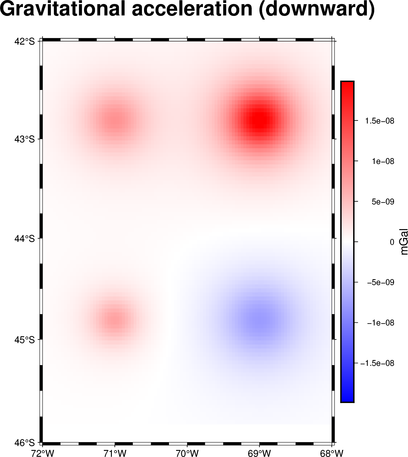
Working with sources defined in geodetic coordinates#
If our point sources and computation points are defined in geodetic
coordinates, we can use the boule.Ellipsoid.geodetic_to_spherical
method to convert them to spherical coordinates and use them to compute their
gravitational field.
Lets define a set point sources in geodetic coordinates and their masses:
longitude = np.array([-71, -71, -69, -69])
latitude = np.array([-45, -43, -45, -43])
height = np.array([-10e3, -20e3, -30e3, -20e3])
points = (longitude, latitude, height)

masses = np.array([1e6, 2e6, -3e6, 5e6])
Then, build a regular grid of computation points defined in geodetic coordinates and located at 1km above the ellipsoid:
coordinates = bd.grid_coordinates(
    region=(-72, -68, -46, -42),
    shape=(101, 101),
    non_dimensional_coords=20e3,
)
Before we can start forward modelling these sources, we need to convert them to
spherical coordinates. To do so, we can use the
boule.Ellipsoid.geodetic_to_spherical method:
points_spherical = ellipsoid.geodetic_to_spherical(points)
coordinates_spherical = ellipsoid.geodetic_to_spherical(coordinates)
We can finally use these converted coordinates to compute the gravitational field the source generate on every computation point:
g_z = hm.point_gravity(
    coordinates_spherical,
    points_spherical,
    masses,
    field="g_z",
    coordinate_system="spherical",
)
Lets plot these results using pygmt:
import pygmt

grid = vd.make_xarray_grid(
   coordinates_spherical, g_z, data_names="g_z", extra_coords_names="extra")

fig = pygmt.Figure()
title = "Gravitational acceleration (downward)"
maxabs = vd.maxabs(g_z)*.95
pygmt.makecpt(cmap="polar", series=(-maxabs, maxabs), background=True)

fig.grdimage(
   region=(-72, -68, -46, -42),
   projection="M10c",
   grid=grid.g_z,
   frame=[f"WSne+t{title}", "x", "y"],
   cmap=True,)

fig.colorbar(cmap=True, position="JMR", frame=["a0.000000005", "x+lmGal"])
fig.show()