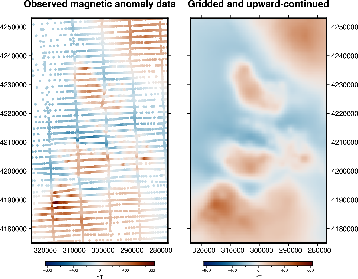
Gridding and upward continuation

Most potential field surveys gather data along scattered and uneven flight lines or ground measurements. For a great number of applications we may need to interpolate these data points onto a regular grid at a constant altitude. Upward-continuation is also a routine task for smoothing, noise attenuation, source separation, etc.

Both tasks can be done simultaneously through an equivalent sources [Dampney1969] (a.k.a equivalent layer). We will use harmonica.EquivalentSources to estimate the coefficients of a set of point sources that fit the observed data. The fitted sources can then be used to predict data values wherever we want, like on a grid at a certain altitude. By default, the sources for EquivalentSources are placed one beneath each data point at a relative depth from the elevation of the data point following [Cordell1992].

The advantage of using equivalent sources is that it takes into account the 3D nature of the observations, not just their horizontal positions. It also allows data uncertainty to be taken into account and noise to be suppressed though the least-squares fitting process. The main disadvantage is the increased computational load (both in terms of time and memory).

Number of data points: 7054
Mean height of observations: 481.34278423589456
R² score: 0.9988825635803776

Generated grid:
 <xarray.Dataset> Size: 241kB
Dimensions:           (northing: 157, easting: 95)
Coordinates:
  * easting           (easting) float64 760B -3.24e+05 -3.235e+05 ... -2.769e+05
  * northing          (northing) float64 1kB 4.175e+06 4.176e+06 ... 4.253e+06
    upward            (northing, easting) float64 119kB 1.5e+03 ... 1.5e+03
Data variables:
    magnetic_anomaly  (northing, easting) float64 119kB 30.7 30.83 ... 149.4
Attributes:
    metadata:  Generated by EquivalentSources(damping=1, depth=1000)

import ensaio
import pandas as pd
import pygmt
import pyproj
import verde as vd

import harmonica as hm

# Fetch the sample total-field magnetic anomaly data from Great Britain
fname = ensaio.fetch_britain_magnetic(version=1)
data = pd.read_csv(fname)

# Slice a smaller portion of the survey data to speed-up calculations for this
# example
region = [-5.5, -4.7, 57.8, 58.5]
inside = vd.inside((data.longitude, data.latitude), region)
data = data[inside]
print("Number of data points:", data.shape[0])
print("Mean height of observations:", data.height_m.mean())

# Since this is a small area, we'll project our data and use Cartesian
# coordinates
projection = pyproj.Proj(proj="merc", lat_ts=data.latitude.mean())
easting, northing = projection(data.longitude.values, data.latitude.values)
coordinates = (easting, northing, data.height_m)
xy_region = vd.get_region((easting, northing))

# Create the equivalent sources.
# We'll use the default point source configuration at a relative depth beneath
# each observation point.
# The damping parameter helps smooth the predicted data and ensure stability.
eqs = hm.EquivalentSources(depth=1000, damping=1)

# Fit the sources coefficients to the observed magnetic anomaly.
eqs.fit(coordinates, data.total_field_anomaly_nt)

# Evaluate the data fit by calculating an R² score against the observed data.
# This is a measure of how well the sources fit the data, NOT how good the
# interpolation will be.
print("R² score:", eqs.score(coordinates, data.total_field_anomaly_nt))

# Interpolate data on a regular grid with 500 m spacing. The interpolation
# requires the height of the grid points (upward coordinate). By passing in
# 1500 m, we're effectively upward-continuing the data (mean flight height is
# 500 m).

grid_coords = vd.grid_coordinates(region=xy_region, spacing=500, extra_coords=1500)

grid = eqs.grid(coordinates=grid_coords, data_names=["magnetic_anomaly"])

# The grid is a xarray.Dataset with values, coordinates, and metadata
print("\nGenerated grid:\n", grid)

# Set figure properties
w, e, s, n = xy_region
fig_height = 10
fig_width = fig_height * (e - w) / (n - s)
fig_ratio = (n - s) / (fig_height / 100)
fig_proj = f"x1:{fig_ratio}"

# Plot original magnetic anomaly and the gridded and upward-continued version
fig = pygmt.Figure()

title = "Observed magnetic anomaly data"

# Make colormap of data
# Get the 95 percentile of the maximum absolute value between the original and
# gridded data so we can use the same color scale for both plots and have 0
# centered at the white color.
maxabs = vd.maxabs(data.total_field_anomaly_nt, grid.magnetic_anomaly.values) * 0.95
pygmt.makecpt(
    cmap="vik",
    series=(-maxabs, maxabs),
    background=True,
)

with pygmt.config(FONT_TITLE="12p"):
    fig.plot(
        projection=fig_proj,
        region=xy_region,
        frame=[f"WSne+t{title}", "xa10000", "ya10000"],
        x=easting,
        y=northing,
        fill=data.total_field_anomaly_nt,
        style="c0.1c",
        cmap=True,
    )

fig.colorbar(cmap=True, frame=["a400f100", "x+lnT"])

fig.shift_origin(xshift=fig_width + 1)

title = "Gridded and upward-continued"

with pygmt.config(FONT_TITLE="12p"):
    fig.grdimage(
        frame=[f"ESnw+t{title}", "xa10000", "ya10000"],
        grid=grid.magnetic_anomaly,
        cmap=True,
    )

fig.colorbar(cmap=True, frame=["a400f100", "x+lnT"])

fig.show()