Tilt of a regular grid

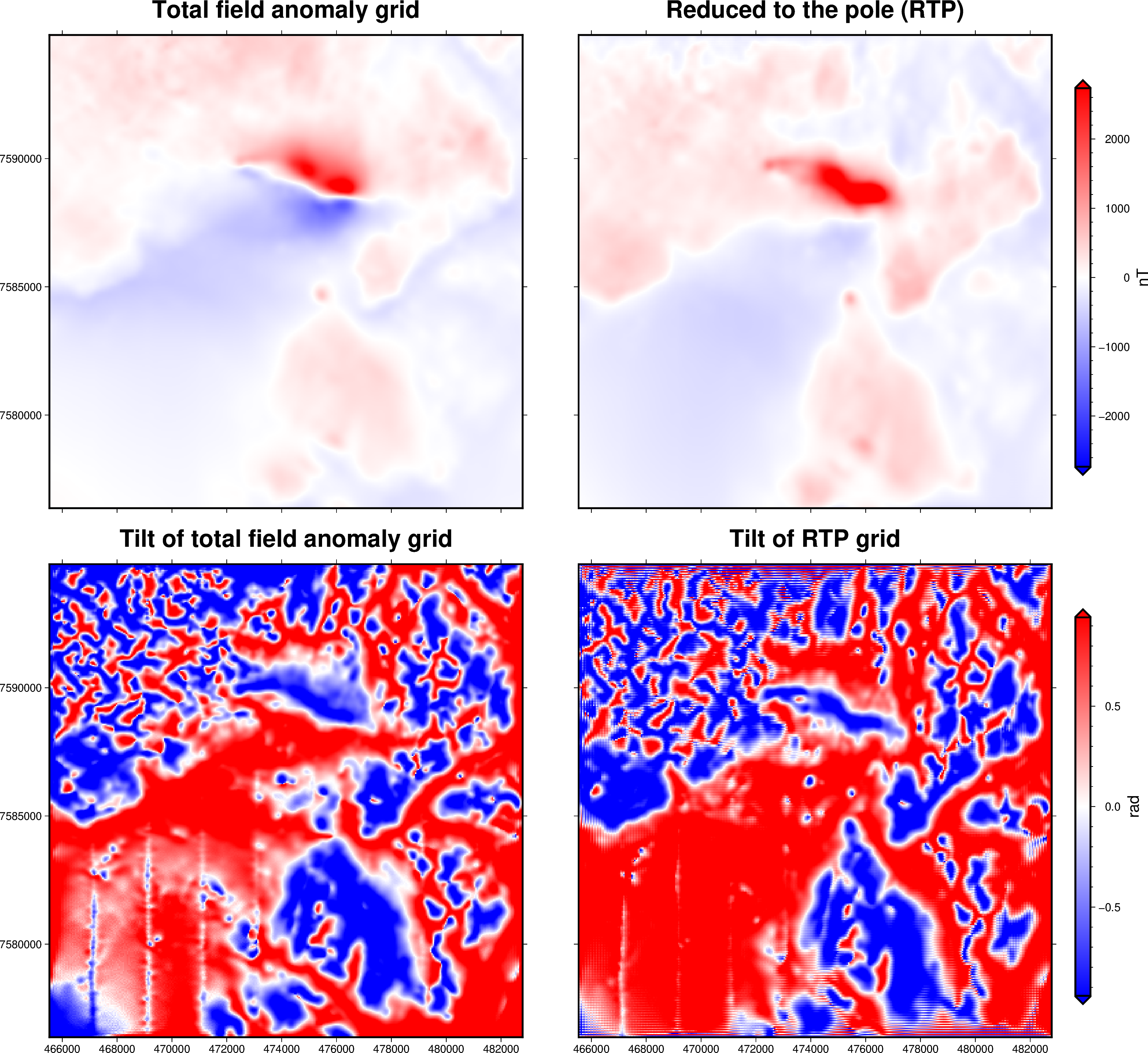
Tilt:
 <xarray.DataArray (northing: 370, easting: 346)> Size: 1MB
array([[ 0.10172001, -0.74481704, -0.93128415, ..., -0.99887809,
        -0.98479112, -1.09844667],
       [-0.90766593, -1.22480118, -1.29916495, ..., -0.75158608,
        -0.72044571, -0.92884452],
       [-1.07462382, -1.36087411, -1.49481561, ..., -0.70429216,
        -0.70897604, -0.85844459],
       ...,
       [-0.87471433, -0.32942091,  0.10326239, ...,  0.29601165,
         0.65236242,  0.9811706 ],
       [-0.92700474, -0.47970142, -0.03181854, ...,  0.26675736,
         0.63699939,  0.97524498],
       [-0.71785463, -0.22386292,  0.11861764, ...,  0.13753573,
         0.44638079,  0.83413707]], shape=(370, 346))
Coordinates:
  * northing  (northing) float64 3kB 7.576e+06 7.576e+06 ... 7.595e+06 7.595e+06
  * easting   (easting) float64 3kB 4.655e+05 4.656e+05 ... 4.827e+05 4.828e+05
    height    (northing, easting) float64 1MB 500.0 500.0 500.0 ... 500.0 500.0

Tilt from RTP:
 <xarray.DataArray (northing: 370, easting: 346)> Size: 1MB
array([[-1.06450644, -1.45635179, -1.41685023, ..., -0.52955435,
        -0.29100831, -0.56997043],
       [-1.241621  , -1.36914956, -1.33726765, ...,  0.21463618,
         0.47138089,  0.30185597],
       [-0.56799045, -1.00005283, -1.0171184 , ...,  0.64376767,
         0.81315481,  0.58368696],
       ...,
       [-0.79261989, -0.11679551,  0.21194443, ...,  0.53018773,
         0.87937371,  1.09492782],
       [-0.7332206 , -0.07124476,  0.22817914, ...,  0.49177504,
         0.83321286,  1.05876888],
       [-0.68345463,  0.02621577,  0.310723  , ...,  0.63909461,
         0.9252598 ,  1.11166334]], shape=(370, 346))
Coordinates:
  * northing  (northing) float64 3kB 7.576e+06 7.576e+06 ... 7.595e+06 7.595e+06
  * easting   (easting) float64 3kB 4.655e+05 4.656e+05 ... 4.827e+05 4.828e+05
    height    (northing, easting) float64 1MB 500.0 500.0 500.0 ... 500.0 500.0

import ensaio
import pygmt
import verde as vd
import xarray as xr

import harmonica as hm

# Fetch magnetic grid over the Lightning Creek Sill Complex, Australia using
# Ensaio and load it with Xarray
fname = ensaio.fetch_lightning_creek_magnetic(version=1)
magnetic_grid = xr.load_dataarray(fname)

# Compute the tilt of the grid
tilt_grid = hm.tilt_angle(magnetic_grid)
# Show the tilt
print("\nTilt:\n", tilt_grid)

# Define the inclination and declination of the region by the time of the data
# acquisition (1990).
inclination, declination = -52.98, 6.51

# Apply a reduction to the pole over the magnetic anomaly grid. We will assume
# that the sources share the same inclination and declination as the
# geomagnetic field.
rtp_grid = hm.reduction_to_pole(
    magnetic_grid,
    inclination=inclination,
    declination=declination,
    magnetization_inclination=inclination,
    magnetization_declination=declination,
)

# Compute the tilt of the padded rtp grid
tilt_rtp_grid = hm.tilt_angle(rtp_grid)
# Show the tilt from RTP
print("\nTilt from RTP:\n", tilt_rtp_grid)

# Plot original magnetic anomaly, its RTP, and the tilt of both
region = (
    magnetic_grid.easting.values.min(),
    magnetic_grid.easting.values.max(),
    magnetic_grid.northing.values.min(),
    magnetic_grid.northing.values.max(),
)
fig = pygmt.Figure()
with fig.subplot(
    nrows=2,
    ncols=2,
    subsize=("20c", "20c"),
    sharex="b",
    sharey="l",
    margins=["1c", "1c"],
):
    scale = 0.5 * vd.maxabs(magnetic_grid, rtp_grid)
    with fig.set_panel(panel=0):
        # Make colormap of data
        pygmt.makecpt(cmap="polar+h", series=[-scale, scale], background=True)
        # Plot magnetic anomaly grid
        fig.grdimage(
            grid=magnetic_grid,
            projection="X?",
            cmap=True,
            frame=["a", "+tTotal field anomaly grid"],
        )
    with fig.set_panel(panel=1):
        # Make colormap of data
        pygmt.makecpt(cmap="polar+h", series=[-scale, scale], background=True)
        # Plot reduced to the pole magnetic anomaly grid
        fig.grdimage(
            grid=rtp_grid,
            projection="X?",
            cmap=True,
            frame=["a", "+tReduced to the pole (RTP)"],
        )
        # Add colorbar
        label = "nT"
        fig.colorbar(
            frame=f"af+l{label}",
            position="JMR+o1/-0.25c+e",
        )

    scale = 0.6 * vd.maxabs(tilt_grid, tilt_rtp_grid)
    with fig.set_panel(panel=2):
        # Make colormap for tilt (saturate it a little bit)
        pygmt.makecpt(cmap="polar+h", series=[-scale, scale], background=True)
        # Plot tilt
        fig.grdimage(
            grid=tilt_grid,
            projection="X?",
            cmap=True,
            frame=["a", "+tTilt of total field anomaly grid"],
        )
    with fig.set_panel(panel=3):
        # Make colormap for tilt rtp (saturate it a little bit)
        pygmt.makecpt(cmap="polar+h", series=[-scale, scale], background=True)
        # Plot tilt
        fig.grdimage(
            grid=tilt_rtp_grid,
            projection="X?",
            cmap=True,
            frame=["a", "+tTilt of RTP grid"],
        )
        # Add colorbar
        label = "rad"
        fig.colorbar(
            frame=f"af+l{label}",
            position="JMR+o1/-0.25c+e",
        )
fig.show()