Ellipsoid

Harmonica is able to forward model the gravity and magnetic fields of ellipsoids through the harmonica.ellipsoid_gravity and the harmonica.ellipsoid_magnetic functions. The former can forward model the gravity acceleration components generated by ellipsoids with homogeneous density, while the latter can compute the magnetic field due to ellipsoids with homogeneous magnetic susceptibility and remanent magnetization, accounting for self-demagnetization effects.

The ellipsoids must be defined through the harmonica.Ellipsoid class. They are defined in Cartesian coordinates and with arbitrary rotations given by three Tait-Bryan angles (a particular case of Euler angles).

Rotated ellipsoid in the easting-northing-upward coordinate system. The ellipsoid orientation is controlled by three angles: yaw, pitch and roll.

Let’s define a single rotated triaxial ellipsoid:

import harmonica as hm

ellipsoid = hm.Ellipsoid(
    a=3.0,
    b=2.0,
    c=1.0,
    yaw=60.0,
    pitch=15.0,
    center=(-10.0, 30.0, -10.0),
)
ellipsoid

harmonica.Ellipsoid(a=3.0, b=2.0, c=1.0, center=(-10.0, 30.0, -10.0), yaw=60.0, pitch=15.0, roll=0.0)

The a, b, and c are the semiaxes lengths along the easting, northing and upward directions, respectively, before the rotation.

Important

The three semiaxes can be passed in any particular order. For example, we could define an excentric ellipsoid in the upward direction as follows:

hm.Ellipsoid(a=1.0, b=1.0, c=10.0)

Gravity fields

The harmonica.ellipsoid_gravity can compute the gravity acceleration components generated by an homogeneous ellipsoid on any set of observation points. It takes the coordinates of the observation points and the collection of ellipsoids we want to forward model. Those ellipsoids need to have a density physical property in order to be accounted in the forward model.

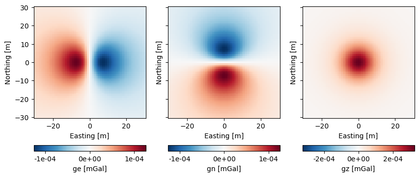
For example, we can define a single ellipsoid with a density contrast of 200 kg/m:sup:3:

ellipsoid = hm.Ellipsoid(
    a=3.0, b=2.0, c=1.0, center=(0.0, 0.0, -10.0), density=200,
)
ellipsoid

harmonica.Ellipsoid(a=3.0, b=2.0, c=1.0, center=(0.0, 0.0, -10.0), yaw=0.0, pitch=0.0, roll=0.0, density=200.0)

And a grid of observation points:

import bordado as bd

coordinates = bd.grid_coordinates(
    region=(-30, 30, -30, 30),
    spacing=1,
    non_dimensional_coords=0,  # height of the grid
)

We can then forward model the ellipsoid:

ge, gn, gz = hm.ellipsoid_gravity(coordinates, ellipsoid)

import verde as vd
import matplotlib.pyplot as plt

_, axes = plt.subplots(nrows=1, ncols=3, sharey=True, figsize=(10, 6))
for ax, g_component, label in zip(
   axes, (ge, gn, gz), ("ge", "gn", "gz"), strict=True
):
    maxabs = vd.maxabs(g_component)
    tmp = ax.pcolormesh(
        coordinates[0],
        coordinates[1],
        g_component,
        vmin=-maxabs,
        vmax=maxabs,
        cmap="RdBu_r",
    )
    plt.colorbar(
        tmp,
        ax=ax,
        label=f"{label} [mGal]",
        orientation="horizontal",
        pad=0.12,
        format='%.0e',
    )
    ax.set_xlabel("Easting [m]")
    ax.set_ylabel("Northing [m]")
    ax.set_aspect("equal")
plt.show()

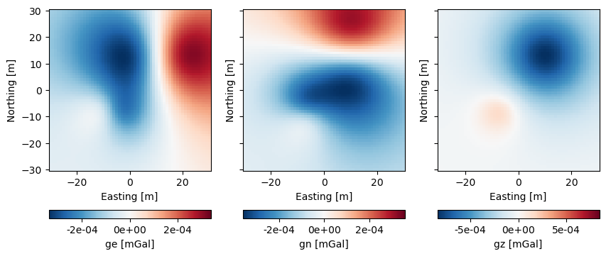
We can also forward model multiple ellipsoid by creating a list of them:

ell_1 = hm.Ellipsoid(
    a=3.0, b=2.0, c=1.0, center=(-7.0, -8.0, -10.0), density=200,
)
ell_2 = hm.Ellipsoid(
    a=2.0, b=4.0, c=5.0, center=(10.0, 13.0, -20.0), density=-300,
)
ellipsoids = [ell_1, ell_2]

ge, gn, gz = hm.ellipsoid_gravity(coordinates, ellipsoids)

_, axes = plt.subplots(nrows=1, ncols=3, sharey=True, figsize=(10, 6))
for ax, g_component, label in zip(
   axes, (ge, gn, gz), ("ge", "gn", "gz"), strict=True
):
    maxabs = vd.maxabs(g_component)
    tmp = ax.pcolormesh(
        coordinates[0],
        coordinates[1],
        g_component,
        vmin=-maxabs,
        vmax=maxabs,
        cmap="RdBu_r",
    )
    plt.colorbar(
        tmp,
        ax=ax,
        label=f"{label} [mGal]",
        orientation="horizontal",
        pad=0.12,
        format='%.0e',
    )
    ax.set_xlabel("Easting [m]")
    ax.set_ylabel("Northing [m]")
    ax.set_aspect("equal")
plt.show()

Tip

If you only need to work with one of the components, you can ignore the other ones using the _ variable name. For example, if we only need the gz component:

_, _, gz = hm.ellipsoid_gravity(coordinates, ellipsoid)

Magnetic fields

The harmonica.ellipsoid_magnetic can compute the magnetic field components generated by an homogeneous ellipsoid on any set of observation points. As in the gravity case, the function takes the coordinates of the observation points, the collection of ellipsoids we want to forward model, and the inducing magnetic field.

The magnetic forward supports ellipsoids that have susceptibility as a physical property. In such case, the inducing magnetic field passed to the function is used to compute its magnetization vector.

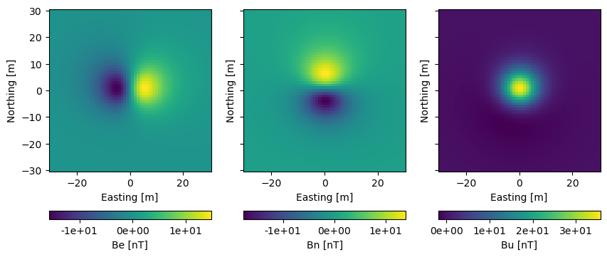
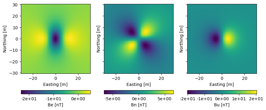
For example, define an ellipsoid with a magnetic susceptibility of 0.2 (in SI units):

ellipsoid = hm.Ellipsoid(
    a=3.0, b=2.0, c=1.0, center=(0.0, 0.0, -10.0), susceptibility=0.2,
)
ellipsoid

harmonica.Ellipsoid(a=3.0, b=2.0, c=1.0, center=(0.0, 0.0, -10.0), yaw=0.0, pitch=0.0, roll=0.0, susceptibility=0.2)

Define the inducing field:

intensity, inc, dec = 55_000.0, -70.0, 15.0
inducing_field = hm.magnetic_angles_to_vec(intensity, inc, dec)

And forward the magnetic field in the grid of observation points:

be, bn, bu = hm.ellipsoid_magnetic(coordinates, ellipsoid, inducing_field)

_, axes = plt.subplots(nrows=1, ncols=3, sharey=True, figsize=(10, 6))
for ax, b_component, label in zip(
   axes, (be, bn, bu), ("Be", "Bn", "Bu"), strict=True
):
    tmp = ax.pcolormesh(coordinates[0], coordinates[1], b_component)
    plt.colorbar(
        tmp,
        ax=ax,
        label=f"{label} [nT]",
        orientation="horizontal",
        pad=0.12,
        format='%.0e',
    )
    ax.set_xlabel("Easting [m]")
    ax.set_ylabel("Northing [m]")
    ax.set_aspect("equal")
plt.show()

Important

The harmonica.ellipsoid_magnetic accounts for the self-demagnetization effect of susceptible ellipsoids. This means that the magnetic fields does not behave linearly with the susceptibility, especially for large susceptibility values.

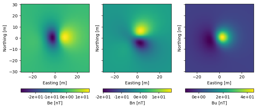
Alternatively, we can specify a remanent magnetization vector to the ellipsoid through the remanent_mag physical property:

remanent_mag = (10.0, 0.0, 0.0)  # in A/m
ellipsoid = hm.Ellipsoid(
    a=3.0, b=2.0, c=1.0, center=(0.0, 0.0, -10.0), remanent_mag=remanent_mag,
)
ellipsoid

harmonica.Ellipsoid(a=3.0, b=2.0, c=1.0, center=(0.0, 0.0, -10.0), yaw=0.0, pitch=0.0, roll=0.0, remanent_mag=[10.  0.  0.])

be, bn, bu = hm.ellipsoid_magnetic(coordinates, ellipsoid, inducing_field)

_, axes = plt.subplots(nrows=1, ncols=3, sharey=True, figsize=(10, 6))
for ax, b_component, label in zip(
   axes, (be, bn, bu), ("Be", "Bn", "Bu"), strict=True
):
    tmp = ax.pcolormesh(coordinates[0], coordinates[1], b_component)
    plt.colorbar(
        tmp,
        ax=ax,
        label=f"{label} [nT]",
        orientation="horizontal",
        pad=0.12,
        format='%.0e',
    )
    ax.set_xlabel("Easting [m]")
    ax.set_ylabel("Northing [m]")
    ax.set_aspect("equal")
plt.show()

Important

The remanent magnetization vector is always aligned with the easting, northing, and upward axes, even if the ellipsoid has rotation angles.

We can even assign both a susceptibility and a remanent magnetization to the ellipsoid:

ellipsoid = hm.Ellipsoid(
    a=3.0,
    b=2.0,
    c=1.0,
    center=(0.0, 0.0, -10.0),
    susceptibility=0.2,
    remanent_mag=remanent_mag,
)
ellipsoid

harmonica.Ellipsoid(a=3.0, b=2.0, c=1.0, center=(0.0, 0.0, -10.0), yaw=0.0, pitch=0.0, roll=0.0, susceptibility=0.2, remanent_mag=[10.  0.  0.])

be, bn, bu = hm.ellipsoid_magnetic(coordinates, ellipsoid, inducing_field)

_, axes = plt.subplots(nrows=1, ncols=3, sharey=True, figsize=(10, 6))
for ax, b_component, label in zip(
   axes, (be, bn, bu), ("Be", "Bn", "Bu"), strict=True
):
    tmp = ax.pcolormesh(coordinates[0], coordinates[1], b_component)
    plt.colorbar(
        tmp,
        ax=ax,
        label=f"{label} [nT]",
        orientation="horizontal",
        pad=0.12,
        format='%.0e',
    )
    ax.set_xlabel("Easting [m]")
    ax.set_ylabel("Northing [m]")
    ax.set_aspect("equal")
plt.show()

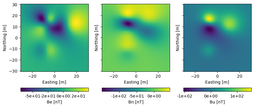
We can also forward a collection of ellipsoids with mixed physical properties:

ell1 = hm.Ellipsoid(
    a=3.0,
    b=2.0,
    c=1.0,
    center=(-8.0, -12.0, -10.0),
    susceptibility=0.3,
)
ell2 = hm.Ellipsoid(
    a=2.0,
    b=5.0,
    c=2.0,
    yaw=35.0,
    roll=10.0,
    center=(-7.0, 13.0, -8.0),
    remanent_mag=(0.0, 10.0, 2.0),
)
ell3 = hm.Ellipsoid(
    a=1.0,
    b=5.0,
    c=6.0,
    pitch=45.0,
    center=(10.0, 9.0, -15.0),
    susceptibility=0.4,
    remanent_mag=(10.0, 10.0, 0.0),
)
ellipsoids = [ell1, ell2, ell3]

be, bn, bu = hm.ellipsoid_magnetic(coordinates, ellipsoids, inducing_field)

_, axes = plt.subplots(nrows=1, ncols=3, sharey=True, figsize=(10, 6))
for ax, b_component, label in zip(
   axes, (be, bn, bu), ("Be", "Bn", "Bu"), strict=True
):
    tmp = ax.pcolormesh(coordinates[0], coordinates[1], b_component)
    plt.colorbar(
        tmp,
        ax=ax,
        label=f"{label} [nT]",
        orientation="horizontal",
        pad=0.12,
        format='%.0e',
    )
    ax.set_xlabel("Easting [m]")
    ax.set_ylabel("Northing [m]")
    ax.set_aspect("equal")
plt.show()