Gradient-boosted equivalent sources

When trying to grid a very large dataset, the regular harmonica.EquivalentSources might not be the best option: they will require a lot of memory for storing the Jacobian matrices involved in the fitting process of the source coefficients. Instead, we can make use of the gradient-boosted equivalent sources, introduced in [Soler2021] and available in Harmonica through the harmonica.EquivalentSourcesGB class. The gradient-boosted equivalent sources divide the survey region in overlapping windows of equal size and fit the source coefficients iteratively, considering the sources and data points that fall under each window at a time. The order in which the windows are visited is randomized to improve convergence of the algorithm.

Here we will produce a grid out of a portion of the ground gravity survey from South Africa (see harmonica.datasets.fetch_south_africa_gravity) using the gradient-boosted equivalent sources. This particlar dataset is not very large, in fact we could use the harmonica.EquivalentSources instead. But we will use the harmonica.EquivalentSourcesGB for illustrating how to use them on a small example.

Number of data points: 6342
Mean height of observations: 868.9293913591926
Required memory for storing the largest Jacobian: 672792 bytes
Number of sources: 6231
R² score: 0.980707030192003
<xarray.Dataset> Size: 3MB
Dimensions:              (northing: 416, easting: 431)
Coordinates:
  * easting              (easting) float64 3kB 1.72e+06 1.722e+06 ... 2.58e+06
  * northing             (northing) float64 3kB -3.495e+06 ... -2.665e+06
    upward               (northing, easting) float64 1MB 1e+03 1e+03 ... 1e+03
Data variables:
    gravity_disturbance  (northing, easting) float64 1MB 7.169 7.235 ... 17.69
Attributes:
    metadata:  Generated by EquivalentSourcesGB(block_size=2000.0, damping=10...

import boule as bl
import ensaio
import pandas as pd
import pygmt
import pyproj
import verde as vd

import harmonica as hm

# Fetch the sample gravity data from South Africa
fname = ensaio.fetch_southern_africa_gravity(version=1)
data = pd.read_csv(fname)

# Slice a smaller portion of the survey data to speed-up calculations for this
# example
region = [18, 27, -34.5, -27]
inside = vd.inside((data.longitude, data.latitude), region)
data = data[inside]
print("Number of data points:", data.shape[0])
print("Mean height of observations:", data.height_sea_level_m.mean())

# Since this is a small area, we'll project our data and use Cartesian
# coordinates
projection = pyproj.Proj(proj="merc", lat_ts=data.latitude.mean())
easting, northing = projection(data.longitude.values, data.latitude.values)
coordinates = (easting, northing, data.height_sea_level_m)
xy_region = vd.get_region((easting, northing))

# Compute the gravity disturbance
ellipsoid = bl.WGS84
data["gravity_disturbance"] = data.gravity_mgal - ellipsoid.normal_gravity(
    data.latitude, data.height_sea_level_m
)

# Create the equivalent sources
# We'll use the block-averaged sources with a block size of 2km and windows of
# 100km x 100km, a damping of 10 and set the sources at a relative depth of
# 9km. By specifying the random_state, we ensure to get the same solution on
# every run.
window_size = 100e3
block_size = 2e3
eqs_gb = hm.EquivalentSourcesGB(
    depth=9e3,
    damping=10,
    window_size=window_size,
    block_size=block_size,
    random_state=42,
)

# Let's estimate the memory required to store the largest Jacobian when using
# these values for the window_size and the block_size.
jacobian_req_memory = eqs_gb.estimate_required_memory(coordinates)
print(f"Required memory for storing the largest Jacobian: {jacobian_req_memory} bytes")

# Fit the sources coefficients to the observed gravity disturbance.
eqs_gb.fit(coordinates, data.gravity_disturbance)

print("Number of sources:", eqs_gb.points_[0].size)

# Evaluate the data fit by calculating an R² score against the observed data.
# This is a measure of how well the sources fit the data, NOT how good the
# interpolation will be.
print("R² score:", eqs_gb.score(coordinates, data.gravity_disturbance))

# Interpolate data on a regular grid with 2 km spacing. The interpolation
# requires the height of the grid points (upward coordinate). By passing in
# 1000 m, we're effectively upward-continuing the data.

grid_coords = vd.grid_coordinates(region=xy_region, spacing=2e3, extra_coords=1000)

grid = eqs_gb.grid(coordinates=grid_coords, data_names="gravity_disturbance")
print(grid)

# Set figure properties
w, e, s, n = xy_region
fig_height = 10
fig_width = fig_height * (e - w) / (n - s)
fig_ratio = (n - s) / (fig_height / 100)
fig_proj = f"x1:{fig_ratio}"

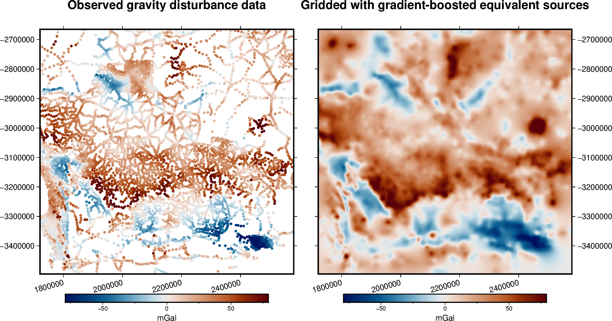
# Plot the original gravity disturbance and the gridded and upward-continued
# version
fig = pygmt.Figure()

title = "Observed gravity disturbance data"

# Make colormap of data
pygmt.makecpt(
    cmap="vik",
    series=(
        -data.gravity_disturbance.quantile(0.99),
        data.gravity_disturbance.quantile(0.99),
    ),
    background=True,
)

with pygmt.config(FONT_TITLE="14p"):
    fig.plot(
        projection=fig_proj,
        region=xy_region,
        frame=[f"WSne+t{title}", "xa200000+a15", "ya100000"],
        x=easting,
        y=northing,
        color=data.gravity_disturbance,
        style="c0.1c",
        cmap=True,
    )

fig.colorbar(cmap=True, frame=["a50f25", "x+lmGal"])

fig.shift_origin(xshift=fig_width + 1)

title = "Gridded with gradient-boosted equivalent sources"

with pygmt.config(FONT_TITLE="14p"):
    fig.grdimage(
        frame=[f"ESnw+t{title}", "xa200000+a15", "ya100000"],
        grid=grid.gravity_disturbance,
        cmap=True,
    )

fig.colorbar(cmap=True, frame=["a50f25", "x+lmGal"])

fig.show()