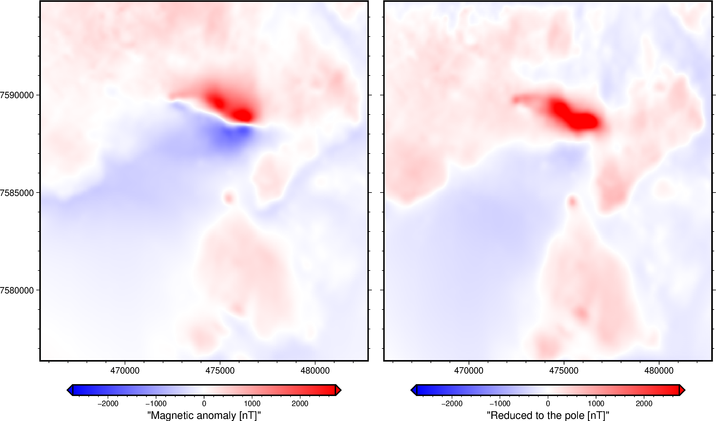
Reduction to the pole of a magnetic anomaly grid

Reduced to the pole magnetic grid:
 <xarray.DataArray (northing: 370, easting: 346)> Size: 1MB
array([[ -47.00485345,  -46.04625474,  -46.18113325, ..., -143.64897504,
        -143.47859109, -142.95056386],
       [ -46.79976423,  -45.95806362,  -46.22151837, ..., -145.37548214,
        -145.2125837 , -144.81709706],
       [ -49.07964615,  -48.24975368,  -48.44025318, ..., -147.16229862,
        -146.93449916, -146.44257154],
       ...,
       [  88.66121321,   71.02597182,   53.23290517, ...,  -73.68480688,
        -115.25167392, -140.59692751],
       [  85.67547575,   69.48843276,   52.69627969, ...,  -76.97781436,
        -117.42227187, -142.21801708],
       [  83.45380812,   67.73864462,   51.48823857, ...,  -83.83587177,
        -122.62522701, -146.42189311]], shape=(370, 346))
Coordinates:
  * northing  (northing) float64 3kB 7.576e+06 7.576e+06 ... 7.595e+06 7.595e+06
  * easting   (easting) float64 3kB 4.655e+05 4.656e+05 ... 4.827e+05 4.828e+05
    height    (northing, easting) float64 1MB 500.0 500.0 500.0 ... 500.0 500.0

import ensaio
import pygmt
import verde as vd
import xarray as xr

import harmonica as hm

# Fetch magnetic grid over the Lightning Creek Sill Complex, Australia using
# Ensaio and load it with Xarray
fname = ensaio.fetch_lightning_creek_magnetic(version=1)
magnetic_grid = xr.load_dataarray(fname)

# Define the inclination and declination of the region by the time of the data
# acquisition (1990).
inclination, declination = -52.98, 6.51

# Apply a reduction to the pole over the magnetic anomaly grid. We will assume
# that the sources share the same inclination and declination as the
# geomagnetic field.
rtp_grid = hm.reduction_to_pole(
    magnetic_grid,
    inclination=inclination,
    declination=declination,
    magnetization_inclination=inclination,
    magnetization_declination=declination,
)
# Show the reduced to the pole grid
print("\nReduced to the pole magnetic grid:\n", rtp_grid)

# Plot original magnetic anomaly and the reduced to the pole
fig = pygmt.Figure()
with fig.subplot(nrows=1, ncols=2, figsize=("28c", "15c"), sharey="l"):
    # Make colormap for both plots (saturate it a little bit)
    scale = 0.5 * vd.maxabs(magnetic_grid, rtp_grid)
    pygmt.makecpt(cmap="polar+h", series=[-scale, scale], background=True)
    with fig.set_panel(panel=0):
        # Plot magnetic anomaly grid
        fig.grdimage(
            grid=magnetic_grid,
            projection="X?",
            cmap=True,
        )
        # Add colorbar
        fig.colorbar(
            frame='af+l"Magnetic anomaly [nT]"',
            position="JBC+h+o0/1c+e",
        )
    with fig.set_panel(panel=1):
        # Plot upward reduced to the pole grid
        fig.grdimage(grid=rtp_grid, projection="X?", cmap=True)
        # Add colorbar
        fig.colorbar(
            frame='af+l"Reduced to the pole [nT]"',
            position="JBC+h+o0/1c+e",
        )
fig.show()