harmonica.point_gravity

harmonica.point_gravity(coordinates, points, masses, field, coordinate_system='cartesian', parallel=True, dtype='float64')

Compute gravitational fields of point masses.

Compute the gravitational potential, gravitational acceleration and tensor components generated by a collection of point masses on a set of observation points defined either in Cartesian or geocentric spherical coordinates.

Warning

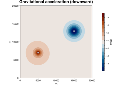
The vertical direction points upwards, i.e. positive and negative values of upward represent points above and below the surface, respectively. But g_z field returns the downward component of the gravitational acceleration so that positive density contrasts produce positive anomalies. The same applies to the tensor components, i.e. the g_ez is the non-diagonal easting-downward tensor component.

Important

• The gravitational potential is returned in \(\text{J}/\text{kg}\).

• The gravity acceleration components are returned in mGal (\(\text{m}/\text{s}^2\)).

• The tensor components are returned in Eotvos (\(\text{s}^{-2}\)).

Parameters:

• coordinates (list of arrays) – List of arrays containing the coordinates of computation points in the following order: easting, northing and upward (if coordinates given in Cartesian coordinates), or longitude, latitude and radius (if given on a spherical geocentric coordinate system). All easting, northing and upward should be in meters. Both longitude and latitude should be in degrees and radius in meters.

• points (list or array) – List or array containing the coordinates of the point masses in the following order: easting, northing and upward (if coordinates given in Cartesian coordinates), or longitude, latitude and radius (if given on a spherical geocentric coordinate system). All easting, northing and upward should be in meters. Both longitude and latitude should be in degrees and radius in meters.

• masses (list or array) – List or array containing the mass of each point mass in kg.

• field (str) –

  Gravitational field that wants to be computed. The available fields coordinates are:

  • Gravitational potential: potential

  • Easting acceleration: g_e

  • Northing acceleration: g_n

  • Downward acceleration: g_z

  • Tensor components:

    • g_ee

    • g_nn

    • g_zz

    • g_en

    • g_ez

    • g_nz

• coordinate_system (str (optional)) – Coordinate system of the coordinates of the computation points and the point masses. Available coordinates systems: cartesian, spherical. Default cartesian.

• parallel (bool (optional)) – If True the computations will run in parallel using Numba built-in parallelization. If False, the forward model will run on a single core. Might be useful to disable parallelization if the forward model is run by an already parallelized workflow. Default to True.

• dtype (data-type (optional)) – Data type assigned to resulting gravitational field. Default to np.float64.

Returns:

result (array) – Gravitational field generated by the point_mass on the computation points defined in coordinates. The potential is given in SI units, the accelerations in mGal and the Marussi tensor components in Eotvos.

Notes

The gravitational potential field generated by a point mass with mass \(m\) located at a point \(Q\) on a computation point \(P\) can be computed as:

\[V(P) = \frac{G m}{l},\]

where \(G\) is the gravitational constant and \(l\) is the Euclidean distance between \(P\) and \(Q\) [Blakely1995].

In Cartesian coordinates, the points \(P\) and \(Q\) are given by \(x\), \(y\) and \(z\) coordinates, which can be translated into northing, easting and upward, respectively. If \(P\) is located at \((x, y, z)\), and \(Q\) at \((x_p, y_p, z_p)\), the distance \(l\) can be computed as:

\[l = \sqrt{ (x - x_p)^2 + (y - y_p)^2 + (z - z_p)^2 }.\]

The gradient of the potential, also known as the gravitational acceleration vector \(\vec{g}\), is defined as:

\[\vec{g} = \nabla V\]

and has components \(g_{northing}(P)\), \(g_{easting}(P)\) and \(g_{upward}(P)\) given by

\[g_{northing}(P) = - \frac{G m}{l^3} (x - x_p),\]

\[g_{easting}(P) = - \frac{G m}{l^3} (y - y_p)\]

and

\[g_{upward}(P) = - \frac{G m}{l^3} (z - z_p).\]

We define the downward component of the gravitational acceleration as the opposite of \(g_{upward}\) (remember that \(z\) points upwards):

\[g_{z}(P) = \frac{G m}{l^3} (z - z_p).\]

On a geocentric spherical coordinate system, the points \(P\) and \(Q\) are given by the longitude, latitude and radius coordinates, i.e. \(\lambda\), \(\varphi\) and \(r\), respectively. On this coordinate system, the Euclidean distance between \(P(r, \varphi, \lambda)\) and \(Q(r_p, \varphi_p, \lambda_p)\) can be calculated as follows [Grombein2013]:

\[l = \sqrt{ r^2 + r_p^2 - 2 r r_p \cos \Psi },\]

where

\[\cos \Psi = \sin \varphi \sin \varphi_p + \cos \varphi \cos \varphi_p \cos(\lambda - \lambda_p).\]

The radial component of the acceleration vector on a local North-oriented system whose origin is located on the point \(P(r, \varphi, \lambda)\) is given by [Grombein2013]:

\[g_r(P) = - \frac{G m}{l^3} (r - r_p \cos \Psi).\]

We define the downward component of the gravitational acceleration \(g_z\) as the opposite of the radial component:

\[g_z(P) = \frac{G m}{l^3} (r - r_p \cos \Psi).\]

Warning

When working in Cartesian coordinates, the z direction points upwards, i.e. positive and negative values of upward represent points above and below the surface, respectively. But remember that the g_z field returns the downward component of the gravitational acceleration.

Warning

When working in geocentric spherical coordinates, remember that the g_z field returns the downward component of the gravitational acceleration on the local North oriented coordinate system. It is equivalent to the opposite of the radial component, therefore it’s positive if the acceleration vector points inside the spheroid.

Examples using harmonica.point_gravity

Point Masses in Cartesian Coordinates

Point Masses in Cartesian Coordinates