Estimating damping and depth parameters¶

When interpolating gravity and magnetic data through the Equivalent Sources technique we need to choose values for some parameters, like the depth at which the sources will be located or the amount of damping that should be applied.

The choice of these hyperparameters can significantly affect the accuracy of the predictions. One way to make this choice could be a visual inspection of the predictions, but that could be tedious and non-objective. Instead, we could estimate these hyperparameters by evaluating the performance of the equivalent sources with different values for each hyperparameter through a cross validation.

Cross-validating equivalent sources¶

Lets start by loading some sample gravity data:

import ensaio
import pandas as pd

fname = ensaio.fetch_bushveld_gravity(version=1)
data = pd.read_csv(fname)
data

	longitude	latitude	height_sea_level_m	height_geometric_m	gravity_mgal	gravity_disturbance_mgal	gravity_bouguer_mgal
0	25.01500	-26.26334	1230.2	1257.474535	978681.38	25.081592	-113.259165
1	25.01932	-26.38713	1297.0	1324.574150	978669.02	24.538158	-122.662101
2	25.02499	-26.39667	1304.8	1332.401322	978669.28	26.526960	-121.339321
3	25.04500	-26.07668	1165.2	1192.107148	978681.08	17.954814	-113.817543
4	25.07668	-26.35001	1262.5	1289.971792	978665.19	12.700307	-130.460126
...	...	...	...	...	...	...	...
3872	31.51500	-23.86333	300.5	312.710241	978776.85	-4.783965	-39.543608
3873	31.52499	-23.30000	280.7	292.686630	978798.55	48.012766	16.602026
3874	31.54832	-23.19333	245.7	257.592670	978803.55	49.161771	22.456674
3875	31.57333	-23.84833	226.8	239.199065	978808.44	5.116904	-20.419870
3876	31.37500	-23.00000	285.6	297.165672	978734.77	5.186926	-25.922627

3877 rows × 7 columns

And project their coordinates using a Mercator projection:

import pyproj

projection = pyproj.Proj(proj="merc", lat_ts=data.latitude.values.mean())
easting, northing = projection(data.longitude.values, data.latitude.values)

coordinates = (easting, northing, data.height_geometric_m.values)

Lets fit the gravity disturbance using equivalent sources and a first guess for the depth and damping parameters.

import harmonica as hm

eqs_first_guess = hm.EquivalentSources(depth=1e3, damping=1)
eqs_first_guess.fit(coordinates, data.gravity_disturbance_mgal)

EquivalentSources(damping=1, depth=1000.0)

In a Jupyter environment, please rerun this cell to show the HTML representation or trust the notebook.
On GitHub, the HTML representation is unable to render, please try loading this page with nbviewer.org.

We can use a cross-validation to evaluate how well these equivalent sources can accurately predict the values of the field on unobserved locations. We will use verde.cross_val_score and then we will compute the mean value of the score obtained after each cross validation.

import numpy as np
import verde as vd

score_first_guess = np.mean(
    vd.cross_val_score(
        eqs_first_guess,
        coordinates,
        data.gravity_disturbance_mgal,
    )
)
score_first_guess

0.8027851941632995

The resulting score corresponds to the R^2. It represents how well the equivalent sources can reproduce the variation of our data. As closer it gets to one, the better the quality of the predictions.

Estimating hyperparameters¶

We saw that we can evaluate the performance of some equivalent sources with some values for the depth and damping parameters through cross validation. Now, lets use it to estimate a set of hyperparameters that produce more accurate predictions. To do so we are going to apply a simple grid search over the depth, damping space, apply cross validation for each pair of values and keeping track of their score.

Lets start by defining some possible values of damping and depth to explore:

dampings = [0.01, 0.1, 1, 10,]
depths = [5e3, 10e3, 20e3, 50e3]

Note

The actual value of the damping is not significant as its order of magnitude. Exploring different powers of ten is a good place to start.

Then we can build a parameter_sets list where each element corresponds to each possible combination of the values of dampings and depths:

import itertools

parameter_sets = [
    dict(damping=combo[0], depth=combo[1])
    for combo in itertools.product(dampings, depths)
]
print("Number of combinations:", len(parameter_sets))
print("Combinations:", parameter_sets)

Number of combinations: 16
Combinations: [{'damping': 0.01, 'depth': 5000.0}, {'damping': 0.01, 'depth': 10000.0}, {'damping': 0.01, 'depth': 20000.0}, {'damping': 0.01, 'depth': 50000.0}, {'damping': 0.1, 'depth': 5000.0}, {'damping': 0.1, 'depth': 10000.0}, {'damping': 0.1, 'depth': 20000.0}, {'damping': 0.1, 'depth': 50000.0}, {'damping': 1, 'depth': 5000.0}, {'damping': 1, 'depth': 10000.0}, {'damping': 1, 'depth': 20000.0}, {'damping': 1, 'depth': 50000.0}, {'damping': 10, 'depth': 5000.0}, {'damping': 10, 'depth': 10000.0}, {'damping': 10, 'depth': 20000.0}, {'damping': 10, 'depth': 50000.0}]

And now we can actually ran one cross validation for each pair of parameters:

equivalent_sources = hm.EquivalentSources()

scores = []
for params in parameter_sets:
    equivalent_sources.set_params(**params)
    score = np.mean(
        vd.cross_val_score(
            equivalent_sources,
            coordinates,
            data.gravity_disturbance_mgal,
        )
    )
    scores.append(score)
scores

[0.9150928326897365,
9142249773027122,
9043905752276586,
8822529497599865,
9158120453861851,
9179260104390441,
9104311266648288,
8751298775892401,
9161113383638326,
919726173084636,
9070261659772815,
8619681875562726,
915820970419046,
917291888715536,
8946173275890276,
8408182949960261]

Once every score has been computed, we can obtain the best score and the corresponding parameters that generate it:

best = np.argmax(scores)
print("Best score:", scores[best])
print("Score with defaults:", score_first_guess)
print("Best parameters:", parameter_sets[best])

Best score: 0.919726173084636
Score with defaults: 0.8027851941632995
Best parameters: {'damping': 1, 'depth': 10000.0}

We have actually improved our score!

Finally, lets grid the gravity disturbance data using the equivalent sources of the first guess and the best ones obtained after cross validation.

Create some equivalent sources out of the best set of parameters:

eqs_best = hm.EquivalentSources(**parameter_sets[best]).fit(
    coordinates, data.gravity_disturbance_mgal
)

And grid the data using the two equivalent sources:

# Define grid coordinates
region = vd.get_region(coordinates)
grid_coords = vd.grid_coordinates(
    region=region,
    spacing=2e3,
    extra_coords=2.5e3,
)

grid_first_guess = eqs_first_guess.grid(grid_coords)
grid = eqs_best.grid(grid_coords)

Lets plot it:

import pygmt

# Set figure properties
w, e, s, n = region
fig_height = 10
fig_width = fig_height * (e - w) / (n - s)
fig_ratio = (n - s) / (fig_height / 100)
fig_proj = f"x1:{fig_ratio}"

maxabs = vd.maxabs(grid_first_guess.scalars, grid.scalars)

fig = pygmt.Figure()

# Make colormap of data
pygmt.makecpt(cmap="polar+h0",series=(-maxabs, maxabs,))

title = "Gravity disturbance with first guess"

fig.grdimage(
   projection=fig_proj,
   region=region,
   frame=[f"WSne+t{title}", "xa100000+a15", "ya100000"],
   grid=grid_first_guess.scalars,
   cmap=True,
)
fig.colorbar(cmap=True, frame=["a50f25", "x+lmGal"])

fig.shift_origin(xshift=fig_width + 1)

title = "Gravity disturbance with best params"

fig.grdimage(
   frame=[f"ESnw+t{title}", "xa100000+a15", "ya100000"],
   grid=grid.scalars,
   cmap=True,
)
fig.colorbar(cmap=True, frame=["a50f25", "x+lmGal"])

fig.show()

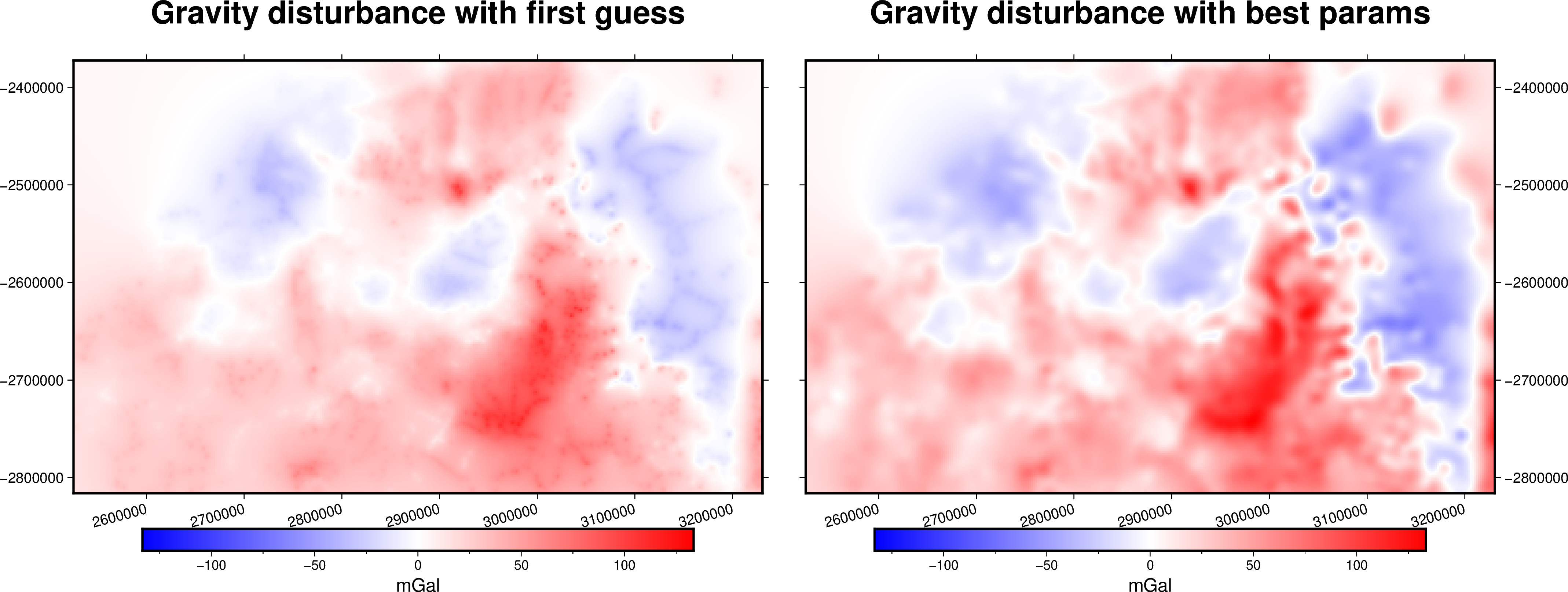
../../_images/eqs-parameters-estimation_10_0.png

The best parameters not only produce a better score, but they also generate a visible more accurate predictions. In the first plot the equivalent sources are so shallow that we can actually see the distribution of sources in the produced grid.

Harmonica v0.6.0

Estimating damping and depth parameters

Contents

Estimating damping and depth parameters¶

Cross-validating equivalent sources¶

Estimating hyperparameters¶