Note
Go to the end to download the full example code
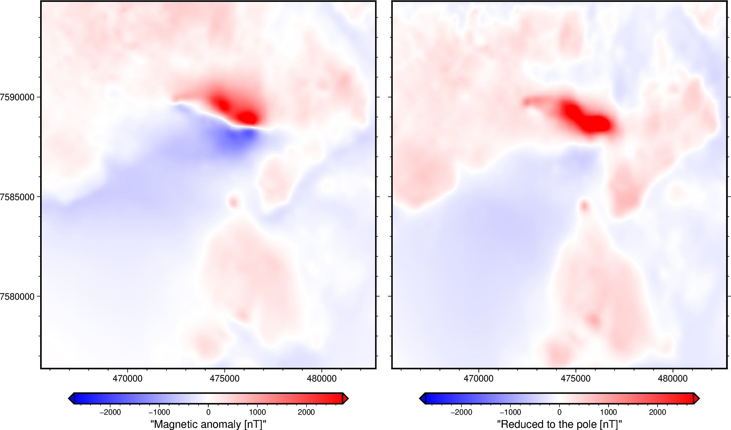
Reduction to the pole of a magnetic anomaly grid#
Reduced to the pole magnetic grid:
 <xarray.DataArray (northing: 370, easting: 346)> Size: 1MB
array([[  14.15546834,   10.38425778,   10.01995891, ..., -219.8102288 ,
        -210.9302948 , -179.38411068],
       [  -3.21249403,   -9.37124449,  -10.96593068, ..., -165.15297526,
        -158.09589683, -133.29346492],
       [  -2.32174677,   -9.44940979,  -11.35233997, ..., -170.79739203,
        -165.2567305 , -141.04626566],
       ...,
       [  45.45701952,  -24.80999268,  -51.27393509, ...,  -40.42602057,
         -64.12371145,  -75.97556295],
       [  36.9104954 ,  -37.13717695,  -58.40650833, ...,  -34.55584156,
         -55.6561726 ,  -71.01718702],
       [-102.42450988, -155.67867833, -165.96638688, ...,  -36.95818214,
         -35.0401052 ,  -40.15055123]])
Coordinates:
  * easting   (easting) float64 3kB 4.655e+05 4.656e+05 ... 4.827e+05 4.828e+05
  * northing  (northing) float64 3kB 7.576e+06 7.576e+06 ... 7.595e+06 7.595e+06
import ensaio
import pygmt
import verde as vd
import xarray as xr
import xrft

import harmonica as hm

# Fetch magnetic grid over the Lightning Creek Sill Complex, Australia using
# Ensaio and load it with Xarray
fname = ensaio.fetch_lightning_creek_magnetic(version=1)
magnetic_grid = xr.load_dataarray(fname)

# Pad the grid to increase accuracy of the FFT filter
pad_width = {
    "easting": magnetic_grid.easting.size // 3,
    "northing": magnetic_grid.northing.size // 3,
}
# drop the extra height coordinate
magnetic_grid_no_height = magnetic_grid.drop_vars("height")
magnetic_grid_padded = xrft.pad(magnetic_grid_no_height, pad_width)

# Define the inclination and declination of the region by the time of the data
# acquisition (1990).
inclination, declination = -52.98, 6.51

# Apply a reduction to the pole over the magnetic anomaly grid. We will assume
# that the sources share the same inclination and declination as the
# geomagnetic field.
rtp_grid = hm.reduction_to_pole(
    magnetic_grid_padded, inclination=inclination, declination=declination
)

# Unpad the reduced to the pole grid
rtp_grid = xrft.unpad(rtp_grid, pad_width)

# Show the reduced to the pole grid
print("\nReduced to the pole magnetic grid:\n", rtp_grid)


# Plot original magnetic anomaly and the reduced to the pole
fig = pygmt.Figure()
with fig.subplot(nrows=1, ncols=2, figsize=("28c", "15c"), sharey="l"):
    # Make colormap for both plots (saturate it a little bit)
    scale = 0.5 * vd.maxabs(magnetic_grid, rtp_grid)
    pygmt.makecpt(cmap="polar+h", series=[-scale, scale], background=True)
    with fig.set_panel(panel=0):
        # Plot magnetic anomaly grid
        fig.grdimage(
            grid=magnetic_grid,
            projection="X?",
            cmap=True,
        )
        # Add colorbar
        fig.colorbar(
            frame='af+l"Magnetic anomaly [nT]"',
            position="JBC+h+o0/1c+e",
        )
    with fig.set_panel(panel=1):
        # Plot upward reduced to the pole grid
        fig.grdimage(grid=rtp_grid, projection="X?", cmap=True)
        # Add colorbar
        fig.colorbar(
            frame='af+l"Reduced to the pole [nT]"',
            position="JBC+h+o0/1c+e",
        )
fig.show()
Total running time of the script: (0 minutes 2.386 seconds)