Equivalent sources in spherical coordinates#

When interpolating gravity or magnetic data over a very large region that covers full continents we need to take into account the curvature of the Earth. In these cases projecting the data to plain Cartesian coordinates may introduce errors due to the distorsions caused by it. Therefore using the harmonica.EquivalentSources class is not well suited for it.

Instead, we can make use of equivalent sources that are defined in spherical geocentric coordinates through the harmonica.EquivalentSourcesSph class.

Lets start by fetching some gravity data over Southern Africa:

import ensaio
import pandas as pd

fname = ensaio.fetch_southern_africa_gravity(version=1)
data = pd.read_csv(fname)
data

	longitude	latitude	height_sea_level_m	gravity_mgal
0	18.34444	-34.12971	32.2	979656.12
1	18.36028	-34.08833	592.5	979508.21
2	18.37418	-34.19583	18.4	979666.46
3	18.40388	-34.23972	25.0	979671.03
4	18.41112	-34.16444	228.7	979616.11
...	...	...	...	...
14354	21.22500	-17.95833	1053.1	978182.09
14355	21.27500	-17.98333	1033.3	978183.09
14356	21.70833	-17.99166	1041.8	978182.69
14357	21.85000	-17.95833	1033.3	978193.18
14358	21.98333	-17.94166	1022.6	978211.38

14359 rows × 4 columns

To speed up the computations on this simple example we are going to downsample the data using a blocked mean to a resolution of 6 arcminutes.

import numpy as np
import verde as vd

blocked_mean = vd.BlockReduce(np.mean, spacing=6 / 60, drop_coords=False)
(longitude, latitude, height), gravity_data = blocked_mean.filter(
    (data.longitude, data.latitude, data.height_sea_level_m),
    data.gravity_mgal,
)

data = pd.DataFrame(
    {
        "longitude": longitude,
        "latitude": latitude,
        "height_sea_level_m": height,
        "gravity_mgal": gravity_data,
    }
)
data

	longitude	latitude	height_sea_level_m	gravity_mgal
0	19.394500	-34.919505	0.00	979750.15
1	19.465000	-34.953000	0.00	979751.50
2	19.554000	-34.996000	0.00	979750.20
3	19.748000	-34.979000	0.00	979747.00
4	19.299585	-34.832660	0.00	979726.95
...	...	...	...	...
8072	15.896660	-17.395000	1104.30	978169.29
8073	15.973330	-17.390000	1106.40	978170.99
8074	16.068330	-17.390000	1110.25	978168.94
8075	16.140000	-17.390000	1112.50	978168.79
8076	18.408330	-17.391660	1115.90	978157.49

8077 rows × 4 columns

And compute gravity disturbance by subtracting normal gravity using boule (see Gravity Disturbance for more information):

import boule as bl

ellipsoid = bl.WGS84
normal_gravity = ellipsoid.normal_gravity(data.latitude, data.height_sea_level_m)
gravity_disturbance = data.gravity_mgal - normal_gravity

Lets define some equivalent sources in spherical coordinates. We will choose some first guess values for the damping and depth parameters.

import harmonica as hm

eqs = hm.EquivalentSourcesSph(damping=1e-3, relative_depth=10000)

See also

Check how we can estimate the damping and depth parameters using a cross-validation.

Before we can fit the sources’ coefficients we need to convert the data given in geographical coordinates to spherical ones. We can do it through the boule.Ellipsoid.geodetic_to_spherical method of the WGS84 ellipsoid defined in boule.

coordinates = ellipsoid.geodetic_to_spherical(
    data.longitude, data.latitude, data.height_sea_level_m
)

And then use them to fit the sources:

eqs.fit(coordinates, gravity_disturbance)

EquivalentSourcesSph(damping=0.001, relative_depth=10000)

In a Jupyter environment, please rerun this cell to show the HTML representation or trust the notebook.
On GitHub, the HTML representation is unable to render, please try loading this page with nbviewer.org.

We can then use these sources to predict the gravity disturbance on a regular grid defined in geodetic coordinates. We will generate a regular grid of computation points located at the maximum height of the data and with a spacing of 6 arcminutes.

# Get the bounding region of the data in geodetic coordinates
region = vd.get_region((data.longitude, data.latitude))

# Get the maximum height of the data coordinates
max_height = data.height_sea_level_m.max()

# Define a regular grid of points in geodetic coordinates
grid_coords = vd.grid_coordinates(
    region=region, spacing=6 / 60, extra_coords=max_height
)

But before we can tell the equivalent sources to predict the field we need to convert the grid coordinates to spherical.

grid_coords_sph = ellipsoid.geodetic_to_spherical(*grid_coords)

And then predict the gravity disturbance on the grid points:

gridded_disturbance = eqs.predict(grid_coords_sph)

Lastly we can generate a xarray.DataArray using verde.make_xarray_grid:

Since the data points don’t cover the entire area, we might want to mask those grid points that are too far away from any data point:

grid = vd.distance_mask(
    data_coordinates=(data.longitude, data.latitude), maxdist=0.5, grid=grid
)

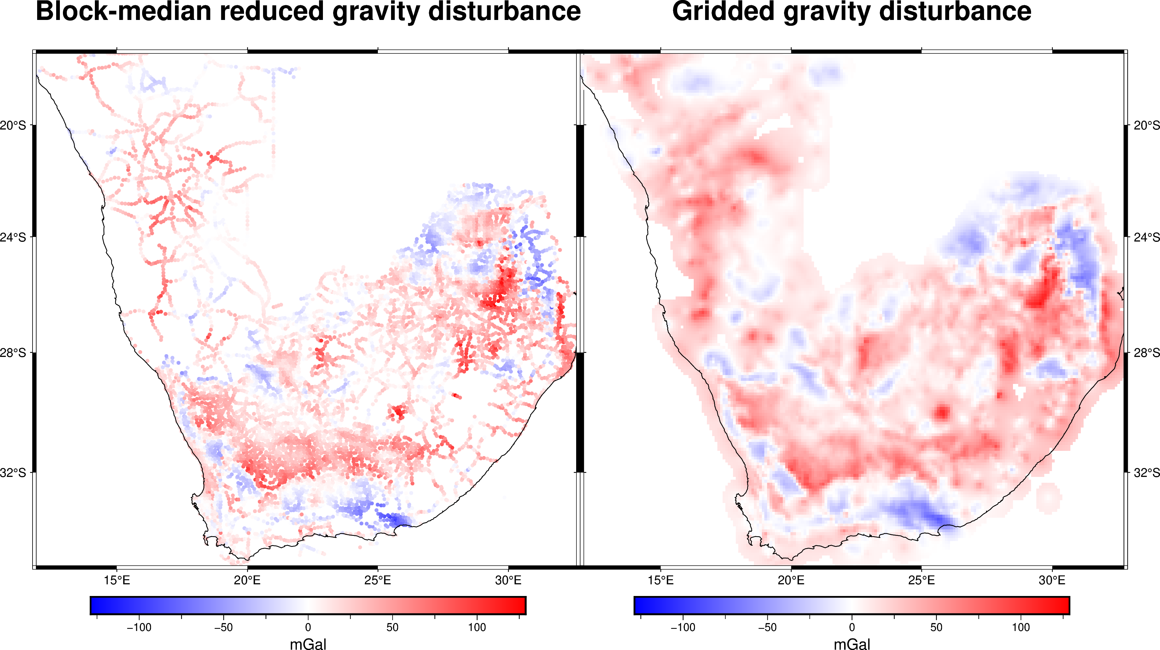
Lets plot it:

import pygmt

maxabs = vd.maxabs(gravity_disturbance, grid.gravity_disturbance.values)

fig = pygmt.Figure()

# Make colormap of data
pygmt.makecpt(cmap="polar+h0",series=(-maxabs, maxabs,))

title = "Block-median reduced gravity disturbance"
fig.plot(
    projection="M100/15c",
    region=region,
    frame=[f"WSne+t{title}", "xa5", "ya4"],
    x=longitude,
    y=latitude,
    fill=gravity_disturbance,
    style="c0.1c",
    cmap=True,
)
fig.coast(shorelines="0.5p,black", area_thresh=1e4)
fig.colorbar(cmap=True, frame=["a50f25", "x+lmGal"])

fig.shift_origin(xshift='w+3c')

title = "Gridded gravity disturbance"
fig.grdimage(
    grid=grid.gravity_disturbance,
    cmap=True,
    frame=[f"ESnw+t{title}","xa5", "ya4"],
    nan_transparent=True,
)
fig.coast(shorelines="0.5p,black", area_thresh=1e4)
fig.colorbar(cmap=True, frame=["a50f25", "x+lmGal"])

fig.show()

../../_images/eq-sources-spherical_12_0.png

Download Python script

Download Jupyter notebook