Toggle navigation

.rst .pdf

repository open issue suggest edit

Gridding with block-averaged equivalent sources

By default, the harmonica.EquivalentSources class locates one point source beneath each data point during the fitting process. Alternatively, we can use another strategy: the block-averaged sources, introduced in [Soler2021].

This method divides the survey region (defined by the data) into square blocks of equal size, computes the median coordinates of the data points that fall inside each block and locates one source beneath every averaged position. This way, we define one equivalent source per block, with the exception of empty blocks that won’t get any source.

This method has two main benefits:

• It lowers the amount of sources involved in the interpolation, therefore it reduces the computer memory requirements and the computation time of the fitting and prediction processes.

• It might avoid to produce aliasing on the output grids, specially for surveys with oversampling along a particular direction, like airborne ones.

We can make use of the block-averaged sources within the harmonica.EquivalentSources class by passing a value to the block_size parameter, which controls the size of the blocks. We recommend using a block_size not larger than the desired resolution of the interpolation grid.

The depth of the sources can be set analogously to the regular equivalent sources: we can use a constant depth (every source is located at the same depth) or a relative depth (where each source is located at a constant shift beneath the median location obtained during the block-averaging process). The depth of the sources and which strategy to use can be set up through the depth and the depth_type parameters, respectively.

Out:

Number of data points: 7054
Mean height of observations: 481.34278423589456
R² score: 0.9958824416327211

Generated grid:
 <xarray.Dataset>
Dimensions:           (northing: 157, easting: 95)
Coordinates:
  * easting           (easting) float64 -3.24e+05 -3.235e+05 ... -2.769e+05
  * northing          (northing) float64 4.175e+06 4.176e+06 ... 4.253e+06
    upward            (northing, easting) float64 1.5e+03 1.5e+03 ... 1.5e+03
Data variables:
    magnetic_anomaly  (northing, easting) float64 28.68 28.71 ... 167.5 157.7
Attributes:
    metadata:  Generated by EquivalentSources(block_size=500, damping=1, dept...
<IPython.core.display.Image object>

import ensaio
import pandas as pd
import pygmt
import pyproj
import verde as vd

import harmonica as hm

# Fetch the sample total-field magnetic anomaly data from Great Britain
fname = ensaio.fetch_britain_magnetic(version=1)
data = pd.read_csv(fname)

# Slice a smaller portion of the survey data to speed-up calculations for this
# example
region = [-5.5, -4.7, 57.8, 58.5]
inside = vd.inside((data.longitude, data.latitude), region)
data = data[inside]
print("Number of data points:", data.shape[0])
print("Mean height of observations:", data.height_m.mean())

# Since this is a small area, we'll project our data and use Cartesian
# coordinates
projection = pyproj.Proj(proj="merc", lat_ts=data.latitude.mean())
easting, northing = projection(data.longitude.values, data.latitude.values)
coordinates = (easting, northing, data.height_m)
xy_region = vd.get_region((easting, northing))

# Create the equivalent sources.
# We'll use block-averaged sources at a constant depth beneath the observation
# points. We will interpolate on a grid with a resolution of 500m, so we will
# use blocks of the same size. The damping parameter helps smooth the predicted
# data and ensure stability.
eqs = hm.EquivalentSources(depth=1000, damping=1, block_size=500, depth_type="constant")

# Fit the sources coefficients to the observed magnetic anomaly.
eqs.fit(coordinates, data.total_field_anomaly_nt)

# Evaluate the data fit by calculating an R² score against the observed data.
# This is a measure of how well the sources fit the data, NOT how good the
# interpolation will be.
print("R² score:", eqs.score(coordinates, data.total_field_anomaly_nt))

# Interpolate data on a regular grid with 500 m spacing. The interpolation
# requires the height of the grid points (upward coordinate). By passing in
# 1500 m, we're effectively upward-continuing the data (mean flight height is
# 500 m).

grid_coords = vd.grid_coordinates(region=xy_region, spacing=500, extra_coords=1500)

grid = eqs.grid(coordinates=grid_coords, data_names=["magnetic_anomaly"])

# The grid is a xarray.Dataset with values, coordinates, and metadata
print("\nGenerated grid:\n", grid)

# Set figure properties
w, e, s, n = xy_region
fig_height = 10
fig_width = fig_height * (e - w) / (n - s)
fig_ratio = (n - s) / (fig_height / 100)
fig_proj = f"x1:{fig_ratio}"

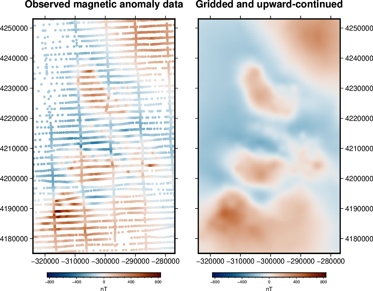
# Plot original magnetic anomaly and the gridded and upward-continued version
fig = pygmt.Figure()

title = "Observed magnetic anomaly data"

# Make colormap of data
# Get the 95 percentile of the maximum absolute value between the original and
# gridded data so we can use the same color scale for both plots and have 0
# centered at the white color.
maxabs = vd.maxabs(data.total_field_anomaly_nt, grid.magnetic_anomaly.values) * 0.95
pygmt.makecpt(
    cmap="vik",
    series=(-maxabs, maxabs),
    background=True,
)

with pygmt.config(FONT_TITLE="12p"):
    fig.plot(
        projection=fig_proj,
        region=xy_region,
        frame=[f"WSne+t{title}", "xa10000", "ya10000"],
        x=easting,
        y=northing,
        color=data.total_field_anomaly_nt,
        style="c0.1c",
        cmap=True,
    )

fig.colorbar(cmap=True, frame=["a400f100", "x+lnT"])

fig.shift_origin(xshift=fig_width + 1)

title = "Gridded and upward-continued"

with pygmt.config(FONT_TITLE="12p"):
    fig.grdimage(
        frame=[f"ESnw+t{title}", "xa10000", "ya10000"],
        grid=grid.magnetic_anomaly,
        cmap=True,
    )

fig.colorbar(cmap=True, frame=["a400f100", "x+lnT"])

fig.show()

previous

Airy Isostatic Moho

next

Gridding and upward continuation