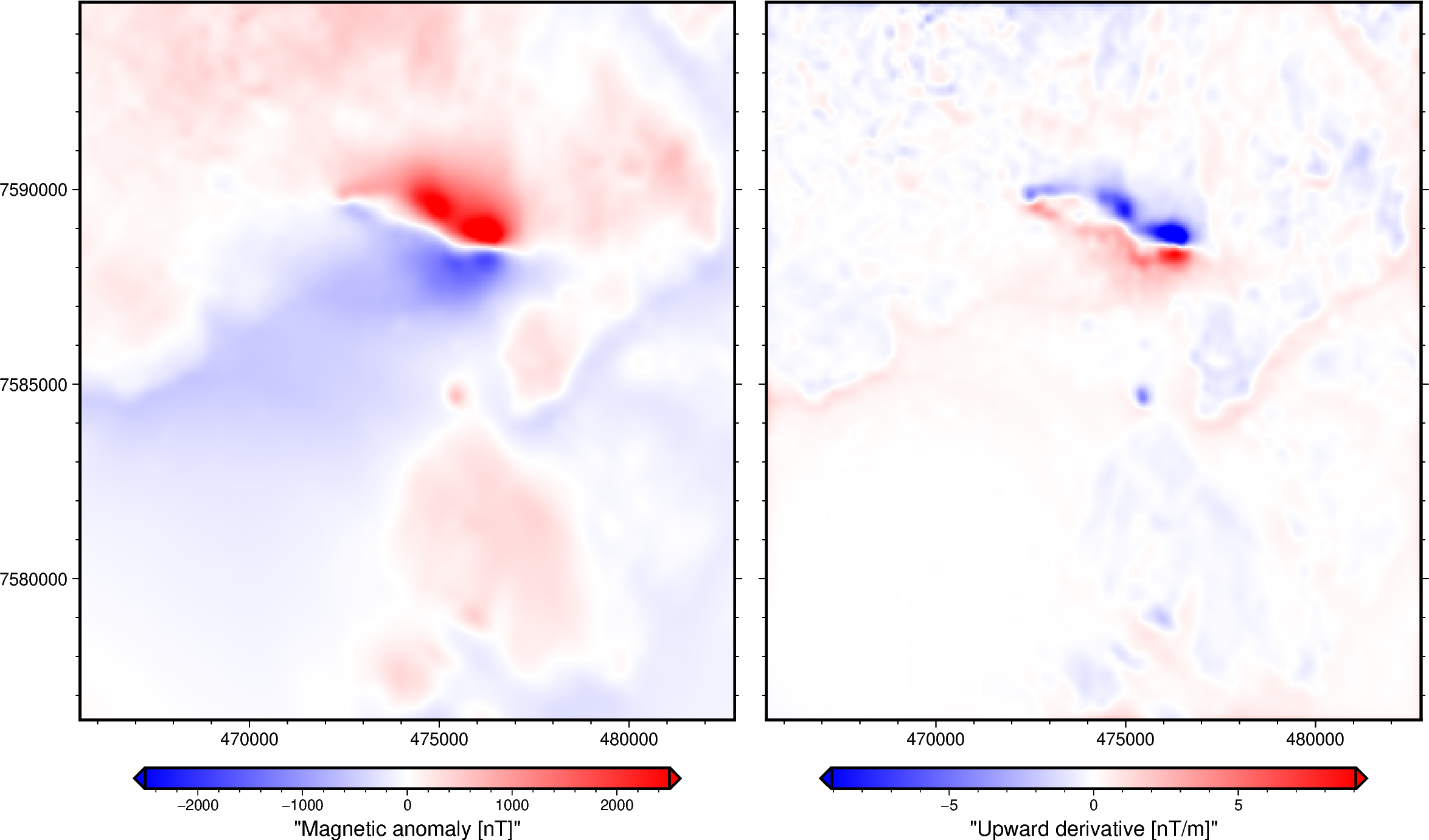
Upward derivative of a regular grid

Upward derivative:
 <xarray.DataArray (northing: 370, easting: 346)> Size: 1MB
array([[-0.95819615, -0.62479717, -0.65249412, ...,  1.73446398,
         1.6766403 ,  2.72435657],
       [-0.63634012, -0.21904971, -0.23107569, ...,  0.49049566,
         0.45948428,  1.68409986],
       [-0.66359177, -0.2353631 , -0.24506233, ...,  0.51034737,
         0.49225437,  1.75482676],
       ...,
       [-3.39466133, -0.92997513, -0.84908229, ...,  0.187395  ,
         0.37947101,  1.13012071],
       [-3.28895188, -0.89679122, -0.84612101, ...,  0.15550382,
         0.36489592,  1.12153698],
       [-5.04820203, -2.9126185 , -2.80733457, ..., -0.11714694,
         0.3870613 ,  1.26040208]])
Coordinates:
  * easting   (easting) float64 3kB 4.655e+05 4.656e+05 ... 4.827e+05 4.828e+05
  * northing  (northing) float64 3kB 7.576e+06 7.576e+06 ... 7.595e+06 7.595e+06

import ensaio
import pygmt
import verde as vd
import xarray as xr
import xrft

import harmonica as hm

# Fetch magnetic grid over the Lightning Creek Sill Complex, Australia using
# Ensaio and load it with Xarray
fname = ensaio.fetch_lightning_creek_magnetic(version=1)
magnetic_grid = xr.load_dataarray(fname)

# Pad the grid to increase accuracy of the FFT filter
pad_width = {
    "easting": magnetic_grid.easting.size // 3,
    "northing": magnetic_grid.northing.size // 3,
}
# drop the extra height coordinate
magnetic_grid_no_height = magnetic_grid.drop_vars("height")
magnetic_grid_padded = xrft.pad(magnetic_grid_no_height, pad_width)

# Compute the upward derivative of the grid
deriv_upward = hm.derivative_upward(magnetic_grid_padded)

# Unpad the derivative grid
deriv_upward = xrft.unpad(deriv_upward, pad_width)

# Show the upward derivative
print("\nUpward derivative:\n", deriv_upward)


# Plot original magnetic anomaly and the upward derivative
fig = pygmt.Figure()
with fig.subplot(nrows=1, ncols=2, figsize=("28c", "15c"), sharey="l"):
    with fig.set_panel(panel=0):
        # Make colormap of data
        scale = 2500
        pygmt.makecpt(cmap="polar+h", series=[-scale, scale], background=True)
        # Plot magnetic anomaly grid
        fig.grdimage(
            grid=magnetic_grid,
            projection="X?",
            cmap=True,
        )
        # Add colorbar
        fig.colorbar(
            frame='af+l"Magnetic anomaly [nT]"',
            position="JBC+h+o0/1c+e",
        )
    with fig.set_panel(panel=1):
        # Make colormap for upward derivative (saturate it a little bit)
        scale = 0.6 * vd.maxabs(deriv_upward)
        pygmt.makecpt(cmap="polar+h", series=[-scale, scale], background=True)
        # Plot upward derivative
        fig.grdimage(grid=deriv_upward, projection="X?", cmap=True)
        # Add colorbar
        fig.colorbar(
            frame='af+l"Upward derivative [nT/m]"',
            position="JBC+h+o0/1c+e",
        )
fig.show()