Equivalent Sources¶

Most potential field surveys gather data along scattered and uneven flight lines or ground measurements. For a great number of applications we may need to interpolate these data points onto a regular grid at a constant altitude. Upward-continuation is also a routine task for smoothing, noise attenuation, source separation, etc.

Both tasks can be done simultaneously through an equivalent sources [Dampney1969] (a.k.a equivalent layer). The equivalent sources technique consists in defining a finite set of geometric bodies (like point sources) beneath the observation points and adjust their coefficients so they generate the same measured field on the observation points. These fitted sources can be then used to predict the values of this field on any unobserved location, like a regular grid, points at different heights, any set of scattered points or even along a profile.

The equivalent sources have two major advantages over any general purpose interpolator:

it takes into account the 3D nature of the potential fields being measured by considering the observation heights, and
its predictions are always harmonic.

Its main drawback is the increased computational load it takes to fit the sources’ coefficients, both in terms of memory and computation time).

Harmonica has a few different classes for applying the equivalent sources techniques. Here we will explore how we can use the harmonica.EquivalentSources to interpolate some gravity disturbance scattered points on a regular grid with a small upward continuation.

We can start by downloading some sample gravity data over the Bushveld Igneous Complex in Southern Africa:

import ensaio
import pandas as pd

fname = ensaio.fetch_bushveld_gravity(version=1)
data = pd.read_csv(fname)
data

	longitude	latitude	height_sea_level_m	height_geometric_m	gravity_mgal	gravity_disturbance_mgal	gravity_bouguer_mgal
0	25.01500	-26.26334	1230.2	1257.474535	978681.38	25.081592	-113.259165
1	25.01932	-26.38713	1297.0	1324.574150	978669.02	24.538158	-122.662101
2	25.02499	-26.39667	1304.8	1332.401322	978669.28	26.526960	-121.339321
3	25.04500	-26.07668	1165.2	1192.107148	978681.08	17.954814	-113.817543
4	25.07668	-26.35001	1262.5	1289.971792	978665.19	12.700307	-130.460126
...	...	...	...	...	...	...	...
3872	31.51500	-23.86333	300.5	312.710241	978776.85	-4.783965	-39.543608
3873	31.52499	-23.30000	280.7	292.686630	978798.55	48.012766	16.602026
3874	31.54832	-23.19333	245.7	257.592670	978803.55	49.161771	22.456674
3875	31.57333	-23.84833	226.8	239.199065	978808.44	5.116904	-20.419870
3876	31.37500	-23.00000	285.6	297.165672	978734.77	5.186926	-25.922627

3877 rows × 7 columns

The harmonica.EquivalentSources class works exclusively in Cartesian coordinates, so we need to project these gravity observations:

import pyproj
import verde as vd

projection = pyproj.Proj(proj="merc", lat_ts=data.latitude.values.mean())
easting, northing = projection(data.longitude.values, data.latitude.values)
region = vd.get_region((easting, northing))

Now we can initialize the harmonica.EquivalentSources class.

import harmonica as hm

equivalent_sources = hm.EquivalentSources(depth=10e3, damping=10)
equivalent_sources

EquivalentSources(damping=10, depth=10000.0)

In a Jupyter environment, please rerun this cell to show the HTML representation or trust the notebook.
On GitHub, the HTML representation is unable to render, please try loading this page with nbviewer.org.

By default, it places the sources one beneath each data point at a relative depth from the elevation of the data point following [Cooper2000]. This relative depth can be set through the depth argument. Deepest sources generate smoother predictions (underfitting), while shallow ones tend to overfit the data.

Note

If instead we want to place every source at a constant depth, we can change it by passing depth_type="constant". In that case, the depth argument will be the exact depth at which the sources will be located.

The damping parameter is used to smooth the coefficients of the sources and stabilize the least square problem. A higher damping will create smoother predictions, while a lower one could overfit the data and create artifacts.

Now we can estimate the source coefficients through the harmonica.EquivalentSources.fit method against the observed gravity disturbance.

coordinates = (easting, northing, data.height_geometric_m)
equivalent_sources.fit(coordinates, data.gravity_disturbance_mgal)

EquivalentSources(damping=10, depth=10000.0)

In a Jupyter environment, please rerun this cell to show the HTML representation or trust the notebook.
On GitHub, the HTML representation is unable to render, please try loading this page with nbviewer.org.

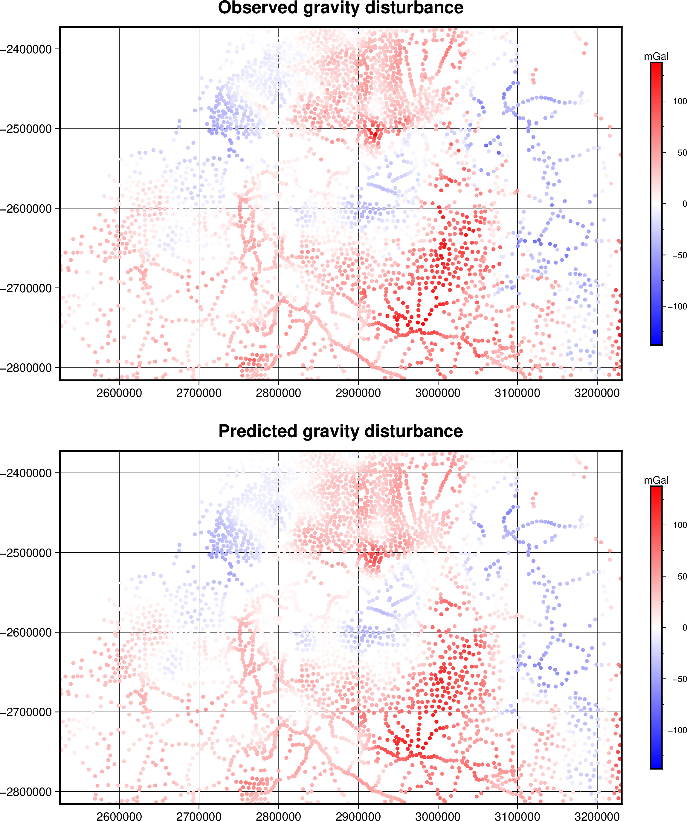
Once the fitting process finishes, we can predict the values of the field on any set of points using the harmonica.EquivalentSources.predict method. For example, lets predict on the same observation points to check if the sources are able to reproduce the observed field.

disturbance = equivalent_sources.predict(coordinates)

And plot it:

import pygmt

# Get max absolute value for the observed gravity disturbance
maxabs = vd.maxabs(data.gravity_disturbance_mgal)

# Set figure properties
w, e, s, n = region
fig_height = 10
fig_width = fig_height * (e - w) / (n - s)
fig_ratio = (n - s) / (fig_height / 100)
fig_proj = f"x1:{fig_ratio}"

fig = pygmt.Figure()
pygmt.makecpt(cmap="polar+h0", series=[-maxabs, maxabs])
title="Predicted gravity disturbance"
with pygmt.config(FONT_TITLE="14p"):
   fig.plot(
      x=easting,
      y=northing,
      color=disturbance,
      cmap=True,
      style="c3p",
      projection=fig_proj,
      region=region,
      frame=['ag', f"+t{title}"],
   )
fig.colorbar(cmap=True, position="JMR", frame=["a50f25", "y+lmGal"])

fig.shift_origin(yshift=fig_height + 2)

title="Observed gravity disturbance"
with pygmt.config(FONT_TITLE="14p"):
   fig.plot(
      x=easting,
      y=northing,
      color=data.gravity_disturbance_mgal,
      cmap=True,
      style="c3p",
      frame=['ag', f"+t{title}"],
   )
fig.colorbar(cmap=True, position="JMR", frame=["a50f25", "y+lmGal"])

fig.show()

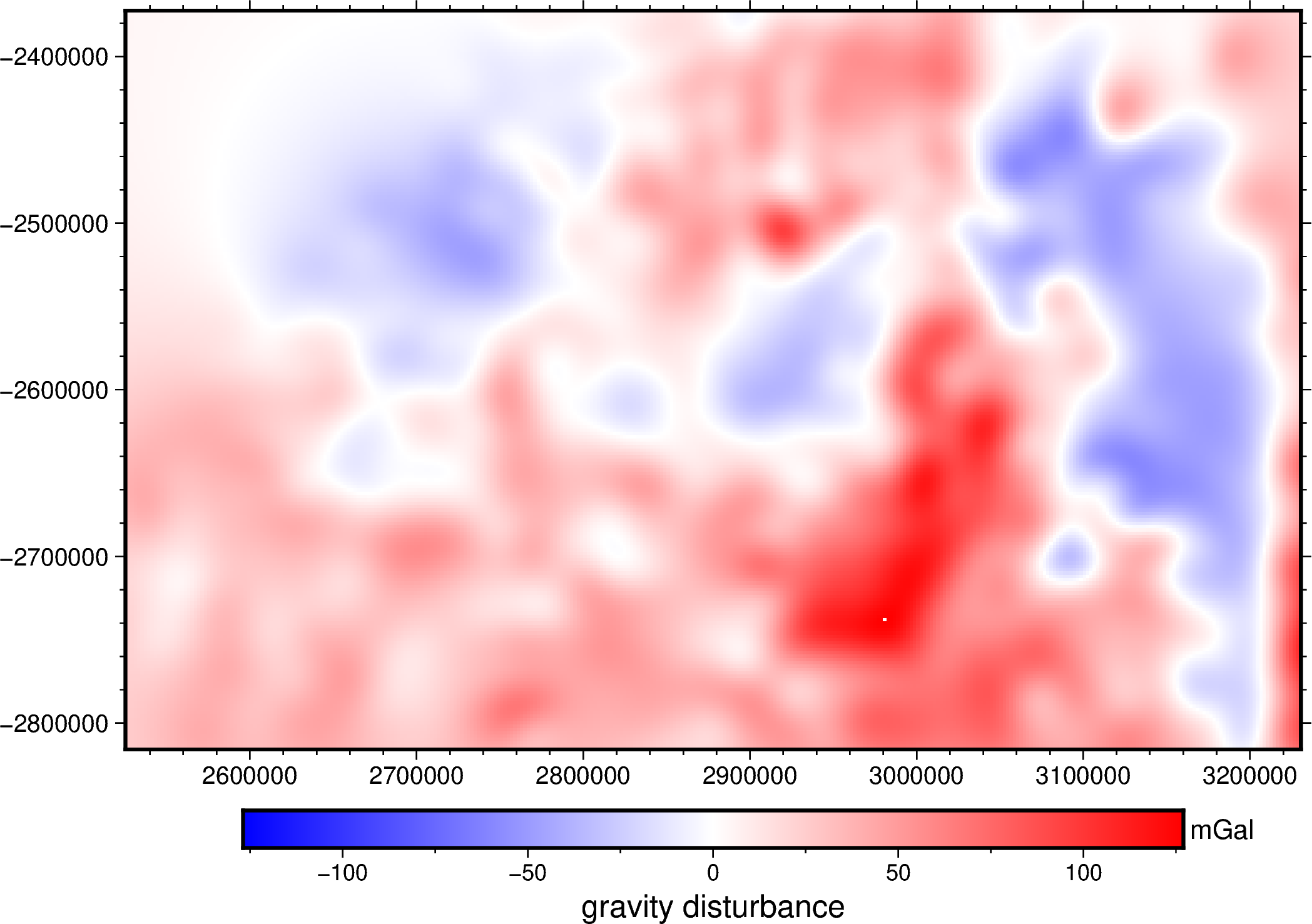
We can also grid and upper continue the field by predicting its values on a regular grid at a constant height higher than the observations. To do so we can use the verde.grid_coordinates function to create the coordinates of the grid and then use the harmonica.EquivalentSources.grid method.

First, lets get the maximum height of the observations:

data.height_geometric_m.max()

2167.498378036602

Then create the grid coordinates at a constant height of and a spacing of 2km; and use the equivalent sources to generate a gravity disturbance grid.

And plot it

maxabs = vd.maxabs(grid.gravity_disturbance)

fig = pygmt.Figure()
pygmt.makecpt(cmap="polar+h0", series=[-maxabs, maxabs])
fig.grdimage(
   frame=['af', 'WSen'],
   grid=grid.gravity_disturbance,
   region=region,
   projection=fig_proj,
   cmap=True,
)
fig.colorbar(cmap=True, frame=["a50f25", "x+lgravity disturbance", "y+lmGal"])

fig.show()

Harmonica v0.6.0

Equivalent Sources

Equivalent Sources¶