Block-averaged equivalent sources¶

When we introduced the Equivalent Sources we saw that by default the harmonica.EquivalentSources class locates one point source beneath each data point during the fitting process, following [Cooper2000].

Alternatively, we can use another strategy: the block-averaged sources, introduced in [Soler2021]. This method divides the survey region (defined by the data) into square blocks of equal size, computes the median coordinates of the data points that fall inside each block and locates one source beneath every averaged position. This way, we define one equivalent source per block, with the exception of empty blocks that won’t get any source.

This method has two main benefits:

It lowers the amount of sources involved in the interpolation, therefore it reduces the computer memory requirements and the computation time of the fitting and prediction processes.
It might avoid to produce aliasing on the output grids, specially for surveys with oversampling along a particular direction, like airborne ones.

We can make use of the block-averaged sources within the harmonica.EquivalentSources class by passing a value to the block_size parameter, which controls the size of the blocks.

Lets load some total-field magnetic data over Great Britain:

import ensaio
import pandas as pd

fname = ensaio.fetch_britain_magnetic(version=1)
data = pd.read_csv(fname)
data

	line_and_segment	year	longitude	latitude	height_m	total_field_anomaly_nt
0	FL1-1	1955	-1.74162	53.48164	792	62
1	FL1-1	1955	-1.70122	53.48352	663	56
2	FL1-1	1955	-1.08051	53.47677	315	30
3	FL1-1	1955	-1.07471	53.47672	315	31
4	FL1-1	1955	-1.01763	53.47586	321	44
...	...	...	...	...	...	...
541503	FL-3(TL10-24)-1	1965	-4.68843	58.26786	1031	64
541504	FL-3(TL10-24)-1	1965	-4.68650	58.26786	1045	74
541505	FL-3(TL10-24)-1	1965	-4.68535	58.26790	1035	94
541506	FL-3(TL10-24)-1	1965	-4.68419	58.26787	1024	114
541507	FL-3(TL10-24)-1	1965	-4.68274	58.26790	1011	120

541508 rows × 6 columns

In order to speed-up calculations we are going to slice a smaller portion of the data:

import verde as vd

region = (-5.5, -4.7, 57.8, 58.5)
inside = vd.inside((data.longitude, data.latitude), region)
data = data[inside]
data

	line_and_segment	year	longitude	latitude	height_m	total_field_anomaly_nt
383858	FL-47-2	1964	-5.38345	57.95592	305	112
383859	FL-47-2	1964	-5.38180	57.95614	305	120
383860	FL-47-2	1964	-5.38011	57.95633	305	150
383861	FL-47-2	1964	-5.37851	57.95658	305	170
383862	FL-47-2	1964	-5.37650	57.95693	305	220
...	...	...	...	...	...	...
538970	FL-16(TL24-36)-6	1965	-4.70304	58.49978	319	162
541490	FL-11-5	1965	-4.88674	58.40691	1056	245
541491	FL-11-5	1965	-4.88377	58.40689	1069	250
541492	FL-11-5	1965	-4.88202	58.40724	1055	245
541493	FL-11-5	1965	-4.88047	58.40728	1041	234

7054 rows × 6 columns

And project the geographic coordiantes to plain Cartesian ones:

import pyproj

projection = pyproj.Proj(proj="merc", lat_ts=data.latitude.mean())
easting, northing = projection(data.longitude.values, data.latitude.values)
coordinates = (easting, northing, data.height_m)
xy_region=vd.get_region(coordinates)

import pygmt

maxabs = vd.maxabs(data.total_field_anomaly_nt)*.8

# Set figure properties
w, e, s, n = xy_region
fig_height = 15
fig_width = fig_height * (e - w) / (n - s)
fig_ratio = (n - s) / (fig_height / 100)
fig_proj = f"x1:{fig_ratio}"

# Plot original magnetic anomaly and the gridded and upward-continued version
fig = pygmt.Figure()

title = "Observed total-field magnetic anomaly"

pygmt.makecpt(
    cmap="polar+h0",
    series=(-maxabs, maxabs),
    background=True,
)

with pygmt.config(FONT_TITLE="12p"):
    fig.plot(
        projection=fig_proj,
        region=xy_region,
        frame=[f"WSne+t{title}", "xa10000", "ya10000"],
        x=easting,
        y=northing,
        color=data.total_field_anomaly_nt,
        style="c0.1c",
        cmap=True,
    )
fig.colorbar(cmap=True, position="JMR", frame=["a200f100", "x+lnT"])
fig.show()

../../_images/block-averaged-eqs_3_0.png

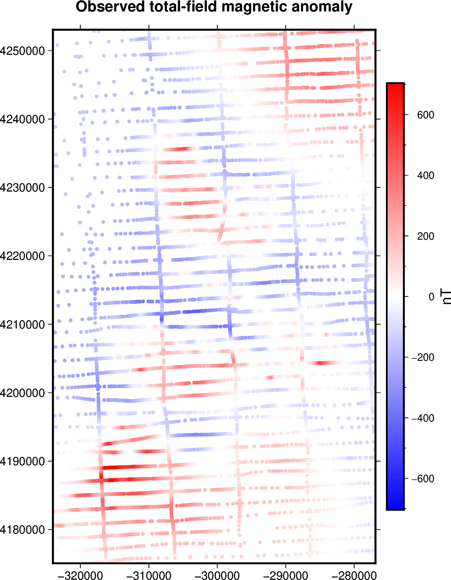
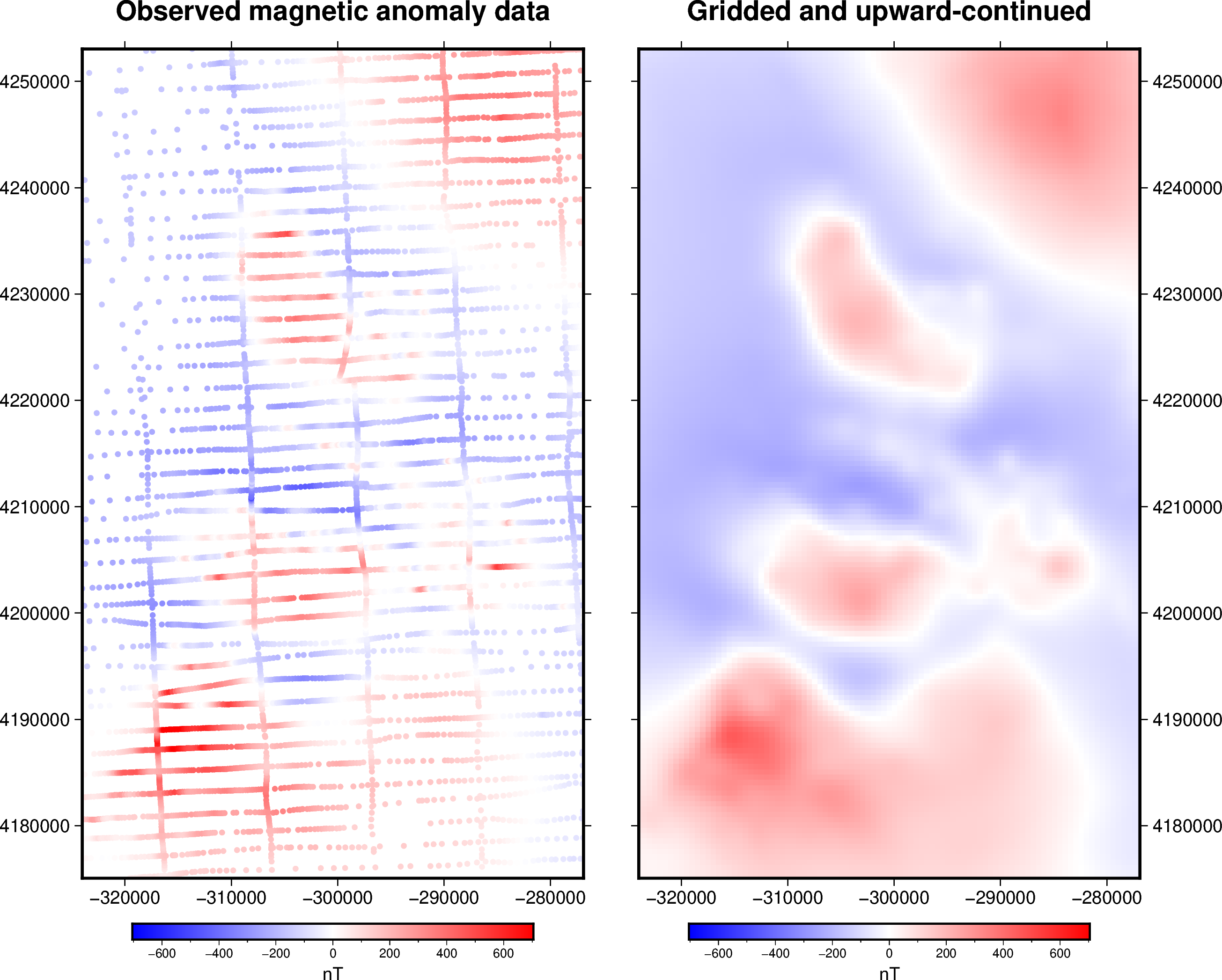
Most airborne surveys like this one present an anysotropic distribution of the data: there are more observation points along the flight lines that goes west to east than the ones going south to north. Placing a single source beneath each observation point generates an anysotropic distribution of the equivalent sources, which might lead to aliases on the generated outputs.

Instead, we can use the block-averaged equivalent sources by creating a harmonica.EquivalentSources instance passing the size of the blocks through the block_size parameter.

import harmonica as hm

eqs = hm.EquivalentSources(
    depth=1000, damping=1, block_size=500, depth_type="constant"
)

These sources were set at a constant depth of 1km bellow the zeroth height and with a damping equal to 1. See how you can choose values for these parameters in Estimating damping and depth parameters.

Note

The depth of the sources can be set analogously to the regular equivalent sources: we can use a constant depth (every source is located at the same depth) or a relative depth (where each source is located at a constant shift beneath the median location obtained during the block-averaging process). The depth of the sources and which strategy to use can be set up through the depth and the depth_type parameters, respectively.

Important

We recommend using a block_size not larger than the desired resolution of the interpolation grid.

Now we can fit the equivalent sources against the magnetic data. During this step the point sources are created through the block averaging process.

eqs.fit(coordinates, data.total_field_anomaly_nt)

EquivalentSources(block_size=500, damping=1, depth=1000, depth_type='constant')

In a Jupyter environment, please rerun this cell to show the HTML representation or trust the notebook.
On GitHub, the HTML representation is unable to render, please try loading this page with nbviewer.org.

Tip

We can obtain the coordinates of the created sources through the points_ attribute. Lets see how many sources it created:

eqs.points_[0].size

We have less sources than observation points indeed.

We can finally grid the magnetic data using the block-averaged equivalent sources. We will generate a regular grid with a resolution of 500 m and at 1500 m height. Since the maximum height of the observation points is around 1000 m we are efectivelly upward continuing the data.

fig = pygmt.Figure()

title = "Observed magnetic anomaly data"
pygmt.makecpt(
    cmap="polar+h0",
    series=(-maxabs, maxabs),
    background=True)

with pygmt.config(FONT_TITLE="14p"):
    fig.plot(
        projection=fig_proj,
        region=xy_region,
        frame=[f"WSne+t{title}", "xa10000", "ya10000"],
        x=easting,
        y=northing,
        color=data.total_field_anomaly_nt,
        style="c0.1c",
        cmap=True,
    )
fig.colorbar(cmap=True, frame=["a200f100", "x+lnT"])

fig.shift_origin(xshift=fig_width + 1)

title = "Gridded and upward-continued"

with pygmt.config(FONT_TITLE="14p"):
    fig.grdimage(
        frame=[f"ESnw+t{title}", "xa10000", "ya10000"],
        grid=grid.magnetic_anomaly,
        cmap=True,
    )
fig.colorbar(cmap=True, frame=["a200f100", "x+lnT"])

fig.show()

../../_images/block-averaged-eqs_8_0.png

Harmonica v0.6.0

Block-averaged equivalent sources

Block-averaged equivalent sources¶