Note
Go to the end to download the full example code
Upward continuation of a regular grid#
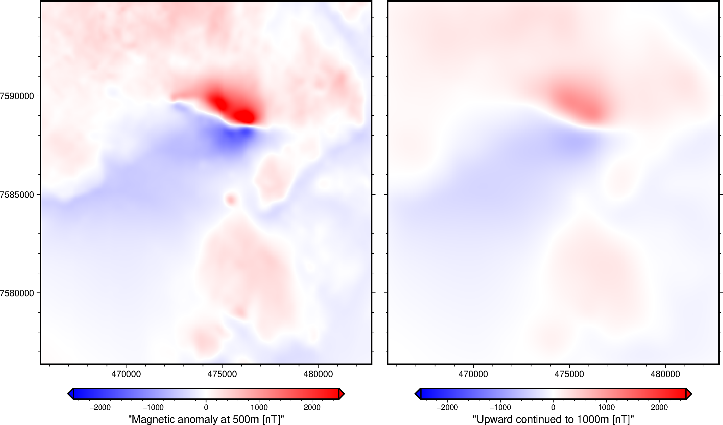
Upward continued magnetic grid:
 <xarray.DataArray (northing: 370, easting: 346)> Size: 1MB
array([[  1.53187928,   1.85099564,   2.13678808, ..., -33.6048979 ,
        -31.65891672, -29.67750887],
       [  1.82032573,   2.17483923,   2.49235855, ..., -35.9639625 ,
        -33.83599574, -31.66680075],
       [  2.07316733,   2.45926837,   2.80498407, ..., -38.27996857,
        -35.97492957, -33.62308159],
       ...,
       [ 50.44855928,  53.84377734,  57.13891805, ...,   4.05301094,
          2.81272119,   1.76442772],
       [ 47.56513259,  50.69950849,  53.74613485, ...,   4.6684348 ,
          3.44419849,   2.39520294],
       [ 44.63682346,  47.50470212,  50.29751413, ...,   5.03755398,
          3.86191533,   2.84250143]])
Coordinates:
  * easting   (easting) float64 3kB 4.655e+05 4.656e+05 ... 4.827e+05 4.828e+05
  * northing  (northing) float64 3kB 7.576e+06 7.576e+06 ... 7.595e+06 7.595e+06
import ensaio
import pygmt
import xarray as xr
import xrft

import harmonica as hm

# Fetch magnetic grid over the Lightning Creek Sill Complex, Australia using
# Ensaio and load it with Xarray
fname = ensaio.fetch_lightning_creek_magnetic(version=1)
magnetic_grid = xr.load_dataarray(fname)

# Pad the grid to increase accuracy of the FFT filter
pad_width = {
    "easting": magnetic_grid.easting.size // 3,
    "northing": magnetic_grid.northing.size // 3,
}
# drop the extra height coordinate
magnetic_grid_no_height = magnetic_grid.drop_vars("height")
magnetic_grid_padded = xrft.pad(magnetic_grid_no_height, pad_width)

# Upward continue the magnetic grid, from 500 m to 1000 m
# (a height displacement of 500m)
upward_continued = hm.upward_continuation(magnetic_grid_padded, height_displacement=500)

# Unpad the upward continued grid
upward_continued = xrft.unpad(upward_continued, pad_width)

# Show the upward continued grid
print("\nUpward continued magnetic grid:\n", upward_continued)


# Plot original magnetic anomaly and the upward continued grid
fig = pygmt.Figure()
with fig.subplot(nrows=1, ncols=2, figsize=("28c", "15c"), sharey="l"):
    # Make colormap for both plots data
    scale = 2500
    pygmt.makecpt(cmap="polar+h", series=[-scale, scale], background=True)
    with fig.set_panel(panel=0):
        # Plot magnetic anomaly grid
        fig.grdimage(
            grid=magnetic_grid,
            projection="X?",
            cmap=True,
        )
        # Add colorbar
        fig.colorbar(
            frame='af+l"Magnetic anomaly at 500m [nT]"',
            position="JBC+h+o0/1c+e",
        )
    with fig.set_panel(panel=1):
        # Plot upward continued grid
        fig.grdimage(grid=upward_continued, projection="X?", cmap=True)
        # Add colorbar
        fig.colorbar(
            frame='af+l"Upward continued to 1000m [nT]"',
            position="JBC+h+o0/1c+e",
        )
fig.show()
Total running time of the script: (0 minutes 0.393 seconds)