Topographic Correction¶

Computing the gravity disturbance is usually the first step towards generating a dataset that could provide insight of the structures and bodies that lie beneath Earth surface.

One of the strongest signals present in the gravity disturbances are the gravitational effect of the topography, i.e. every body located above the surface of the reference ellipsoid. Mainly because their proximity to the observation points but also because their density contrast could be considered the same as their own absolute density.

For this reason, geophysicists usually remove the gravitational effect of the topography from the gravity disturbance in a processes called topographic correction. The resulting field is often called Bouguer gravity disturbance or topography-free gravity disturbance.

The simpler way to apply the topographic correction is through the Bouguer correction. It consists in approximating the topographic masses that lay underneath each computation point as an infinite slab of constant density. It has been widely used on ground surveys because it’s easy to compute and because we don’t need any other data than the observation height (the height at which the gravity has been measured). It’s main drawback is it’s accuracy: the approximation might be too simple to accurately reproduce the gravitational effect of the topography present in our region of interest.

On the other hand, we can compute the topographic correction by forward modelling the topographic masses. To do so we will need a 2D grid of the topography, a.k.a. a DEM (digital elevation model). This method produces accurate corrections if the DEM has good resolutions, but its computation is much more expensive.

In the following sections we will explore how we can apply both methods using Harmonica.

Lets start by downloading some gravity data over the Bushveld Igneous Complex in Southern Africa.

import ensaio
import pandas as pd

fname = ensaio.fetch_bushveld_gravity(version=1)
data = pd.read_csv(fname)
data

	longitude	latitude	height_sea_level_m	height_geometric_m	gravity_mgal	gravity_disturbance_mgal	gravity_bouguer_mgal
0	25.01500	-26.26334	1230.2	1257.474535	978681.38	25.081592	-113.259165
1	25.01932	-26.38713	1297.0	1324.574150	978669.02	24.538158	-122.662101
2	25.02499	-26.39667	1304.8	1332.401322	978669.28	26.526960	-121.339321
3	25.04500	-26.07668	1165.2	1192.107148	978681.08	17.954814	-113.817543
4	25.07668	-26.35001	1262.5	1289.971792	978665.19	12.700307	-130.460126
...	...	...	...	...	...	...	...
3872	31.51500	-23.86333	300.5	312.710241	978776.85	-4.783965	-39.543608
3873	31.52499	-23.30000	280.7	292.686630	978798.55	48.012766	16.602026
3874	31.54832	-23.19333	245.7	257.592670	978803.55	49.161771	22.456674
3875	31.57333	-23.84833	226.8	239.199065	978808.44	5.116904	-20.419870
3876	31.37500	-23.00000	285.6	297.165672	978734.77	5.186926	-25.922627

3877 rows × 7 columns

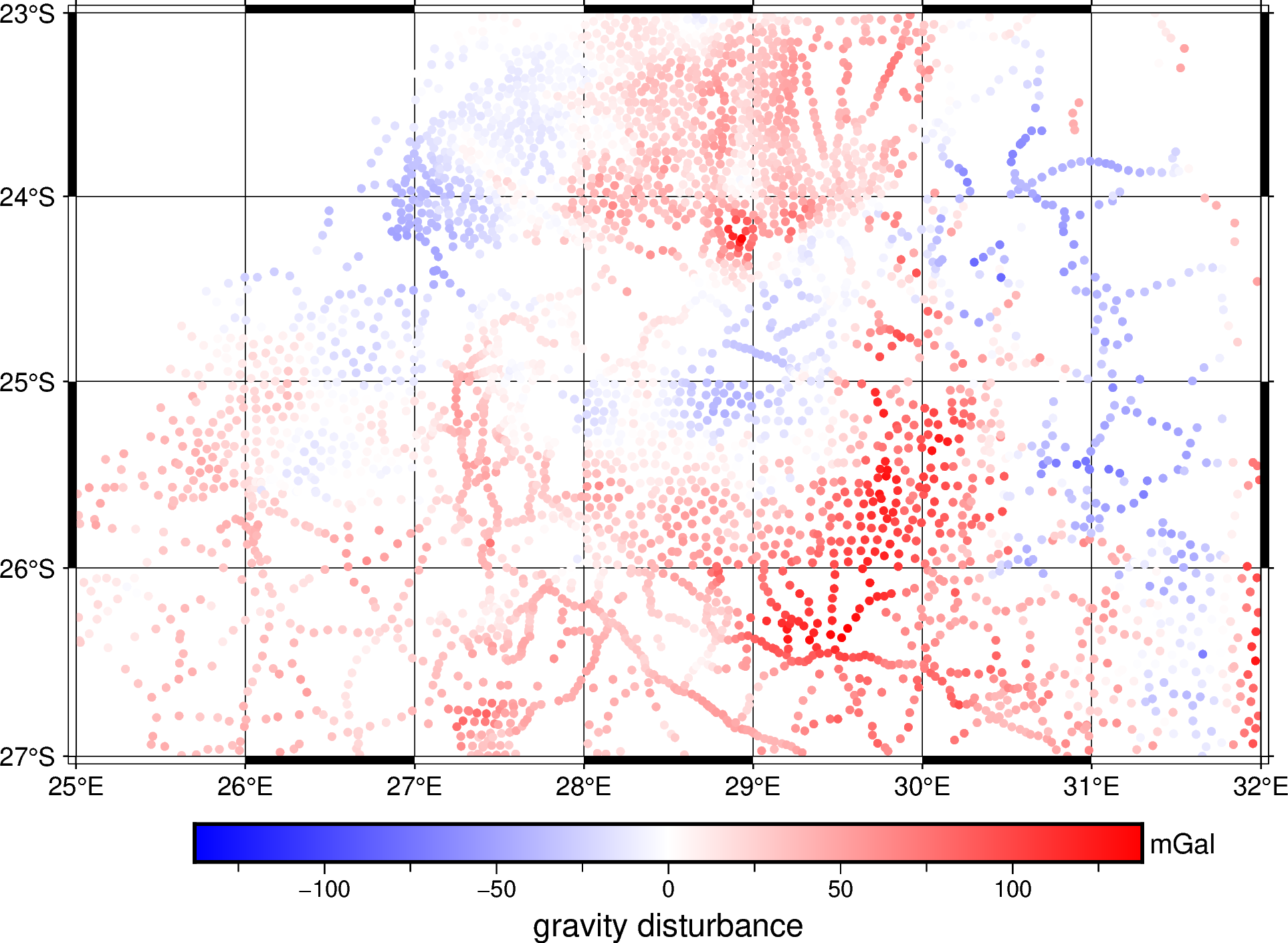
And plot it:

import pygmt
import verde as vd

maxabs = vd.maxabs(data.gravity_disturbance_mgal)

fig = pygmt.Figure()
pygmt.makecpt(cmap="polar+h0", series=[-maxabs, maxabs])
fig.plot(
   x=data.longitude,
   y=data.latitude,
   color=data.gravity_disturbance_mgal,
   cmap=True,
   style="c3p",
   projection="M15c",
   frame=['ag', 'WSen'],
)
fig.colorbar(cmap=True, frame=["a50f25", "x+lgravity disturbance", "y+lmGal"])
fig.show()

../_images/topographic_correction_1_0.png

Bouguer correction¶

We can compute the Bouguer correction through the harmonica.bouguer_correction function. Because our gravity data has been obtained on the Earth surface, the height_geometric_m coordinate coincides with the topographic height at each observation point (referenced above the ellipsoid), so we can pass it as the topography argument.

import harmonica as hm

bouguer_correction = hm.bouguer_correction(data.height_geometric_m)

Hint

The harmonica.bouguer_correction assigns default values for the density of the upper crust and the water.

Warning

In case the observations heights were referenced over the geoid (usually marked as above the mean sea level), it’s advisable to convert them to geometric heights by removing the geoid height.

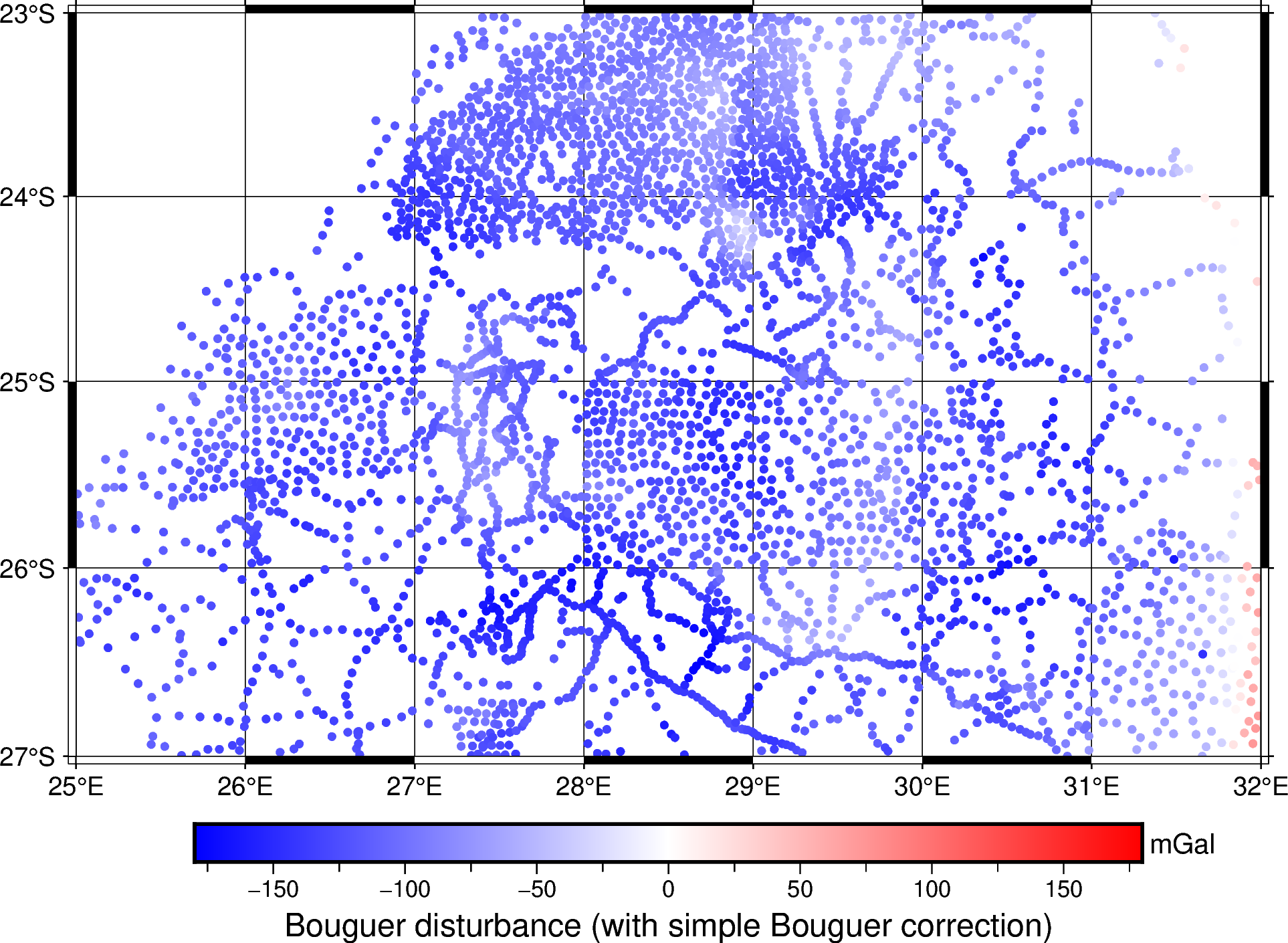
We can now compute the Bouguer disturbance and plot it:

bouguer_disturbance = data.gravity_disturbance_mgal - bouguer_correction
bouguer_disturbance

    -115.688843
    -123.743874
    -122.631301
    -115.497942
    -131.708097
           ...    
  -39.790922
   15.247392
   20.325058
  -21.660701
  -28.079864
Length: 3877, dtype: float64

maxabs = vd.maxabs(bouguer_disturbance)

fig = pygmt.Figure()
pygmt.makecpt(cmap="polar+h0", series=[-maxabs, maxabs])
fig.plot(
   x=data.longitude,
   y=data.latitude,
   color=bouguer_disturbance,
   cmap=True,
   style="c3p",
   projection="M15c",
   frame=['ag', 'WSen'],
)
fig.colorbar(cmap=True, frame=["a50f25", "x+lBouguer disturbance (with simple Bouguer correction)", "y+lmGal"])
fig.show()

../_images/topographic_correction_4_0.png

Forward modelling the topography¶

In order to forward model the topographic masses, we need to build a 3D model made out of simpler geometric bodies. In this case, we are going to use rectangular prisms. Then we will compute the gravitational effect of every prism on each computation point.

To do so, we need a regular grid of the topographic heights (or DEM as in Digital Elevation Model) around the Bushveld Igneous Complex. We can download a global topography grid:

And then crop it to a slightly larger region than the gravity observations:

And project it to plain coordinates using pyproj and verde. We start by defining a Mercator projection:

import pyproj

projection = pyproj.Proj(proj="merc", lat_ts=topography.latitude.values.mean())

And project the grid using verde.project_grid:

Tip

Using the "nearest" method makes the projection process faster than using the "linear" one.

Now we can create a 3D model of the topographic masses using a layer of rectangular prisms. We can use the harmonica.prism_layer function to build it. We also need to assign density values to each prism in the layer. For every prism above the ellipsoid we will set the density of the upper crust (2670 kg/m³), while for each prism below it we will assign the density contrast equal to the density of the water (1040 kg/m³) minus the density of the upper crust.

Now we need to compute the gravitational effect of these prisms on every observation point. We can do it through the harmonica.DatasetAccessorPrismLayer.gravity method. But the coordinates of the observation points must be also projected.

# Project the coordinates of the observation points
easting, northing = projection(data.longitude.values, data.latitude.values)
coordinates = (easting, northing, data.height_geometric_m)

# Compute the terrain effect
terrain_effect = prisms.prism_layer.gravity(coordinates, field="g_z")

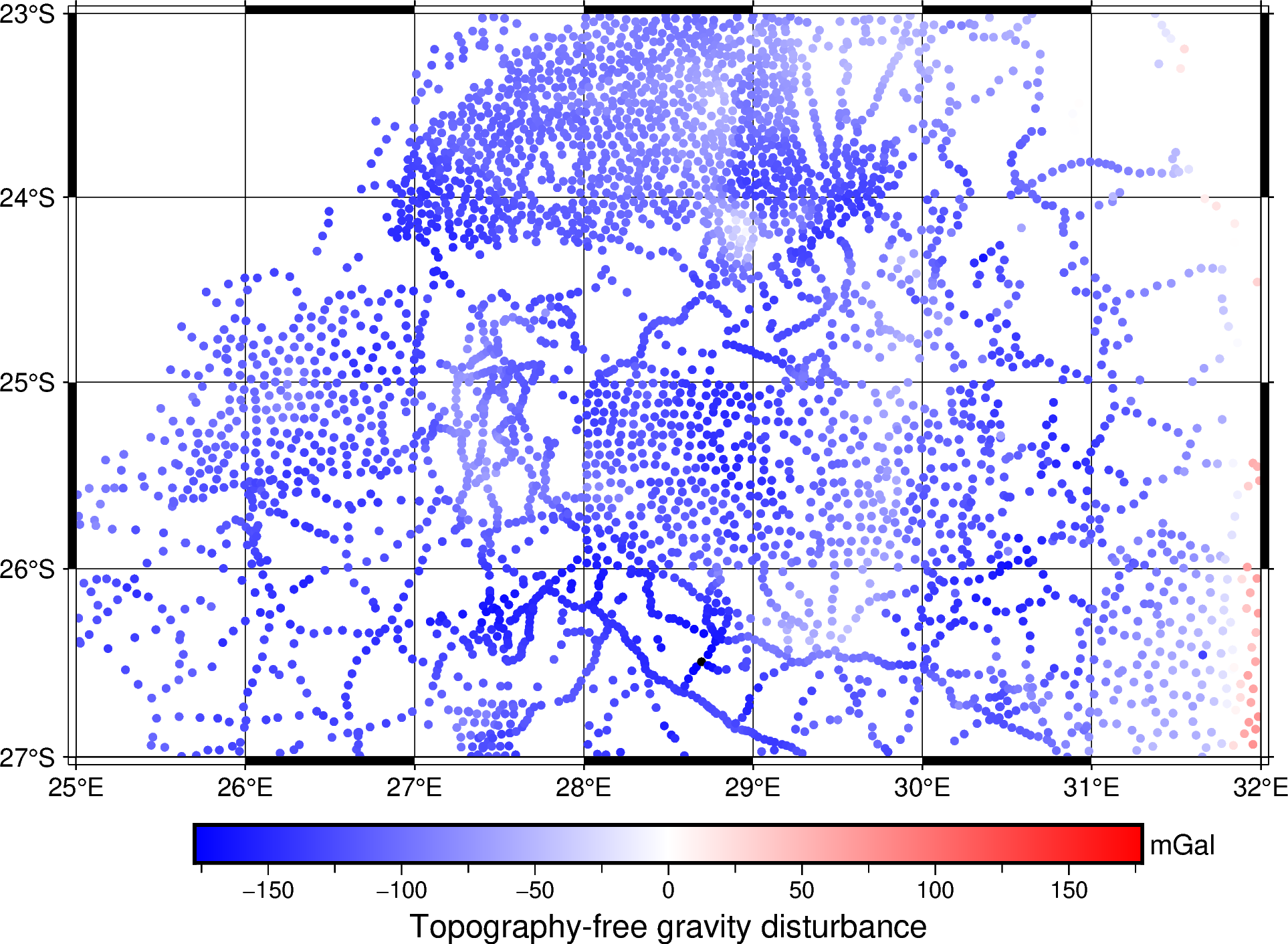
Finally, we can compute the topography-free gravity disturbance:

topo_free_disturbance = data.gravity_disturbance_mgal - terrain_effect

And plot it:

maxabs = vd.maxabs(topo_free_disturbance)

fig = pygmt.Figure()
pygmt.makecpt(cmap="polar+h0", series=[-maxabs, maxabs])
fig.plot(
   x=data.longitude,
   y=data.latitude,
   color=topo_free_disturbance,
   cmap=True,
   style="c3p",
   projection="M15c",
   frame=['ag', 'WSen'],
)
fig.colorbar(cmap=True, frame=["a50f25", "x+lTopography-free gravity disturbance", "y+lmGal"])
fig.show()

../_images/topographic_correction_12_0.png

Harmonica v0.6.0

Topographic Correction

Contents

Topographic Correction¶

Bouguer correction¶

Forward modelling the topography¶