Grid transformations#
Harmonica offers some functions to apply FFT-based (Fast Fourier Transform) and finite-differences transformations to regular grids of gravity and magnetic fields located at a constant height.
In order to apply these grid transformations, we first need a regular grid in
Cartesians coordinates.
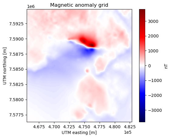
Let’s download a magnetic anomaly grid over the Lightning Creek Sill Complex,
Australia, readily available in ensaio.
We can load the data file using xarray:
import ensaio
import xarray as xr

fname = ensaio.fetch_lightning_creek_magnetic(version=1)
magnetic_grid = xr.load_dataarray(fname)
magnetic_grid
<xarray.DataArray 'total_field_anomaly' (northing: 370, easting: 346)> Size: 1MB
array([[  34.99995117,   36.19995117,   36.69995117, ..., -101.10004883,
        -100.40004883,  -99.60004883],
       [  36.49995117,   37.59995117,   37.99995117, ..., -102.20004883,
        -101.50004883, -100.70004883],
       [  37.09995117,   38.19995117,   38.59995117, ..., -103.30004883,
        -102.60004883, -101.90004883],
       ...,
       [ 182.79995117,  172.39995117,  160.79995117, ...,    0.79995117,
         -24.20004883,  -41.80004883],
       [ 182.09995117,  172.59995117,  161.39995117, ...,    5.99995117,
         -21.50004883,  -41.00004883],
       [ 178.79995117,  170.39995117,  160.29995117, ...,   11.39995117,
         -16.00004883,  -35.80004883]])
Coordinates:
  * easting   (easting) float64 3kB 4.655e+05 4.656e+05 ... 4.827e+05 4.828e+05
  * northing  (northing) float64 3kB 7.576e+06 7.576e+06 ... 7.595e+06 7.595e+06
    height    (northing, easting) float64 1MB 500.0 500.0 500.0 ... 500.0 500.0
Attributes:
    Conventions:   CF-1.8
    title:         Magnetic total-field anomaly of the Lightning Creek sill c...
    crs:           proj=utm zone=54 south datum=WGS84 units=m no_defs ellps=W...
    source:        Interpolated from airborne magnetic line data using gradie...
    license:       Creative Commons Attribution 4.0 International Licence
    references:    Geophysical Acquisition & Processing Section 2019. MIM Dat...
    long_name:     total-field magnetic anomaly
    units:         nT
actual_range: [-1785. 3798.]And plot it:
import matplotlib.pyplot as plt

tmp = magnetic_grid.plot(cmap="seismic", center=0, add_colorbar=False)
plt.gca().set_aspect("equal")
plt.title("Magnetic anomaly grid")
plt.gca().ticklabel_format(style="sci", scilimits=(0, 0))
plt.colorbar(tmp, label="nT")
plt.show()
See also
In case we have a regular grid defined in geographic coordinates (longitude,
latitude) we can project them to Cartesian coordinates using the
verde.project_grid function and a map projection like the ones
available in pyproj.
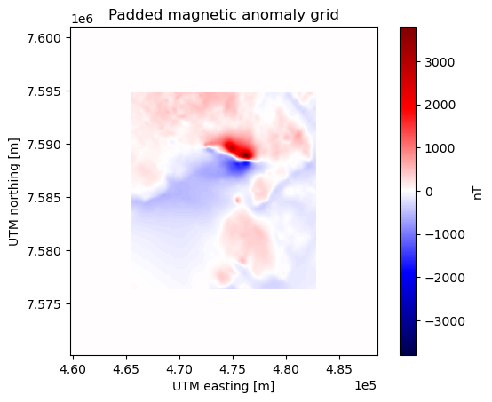
Since all the grid transformations we are going to apply are based on FFT
methods, we usually want to pad them in order their increase the accuracy.
We can easily do it through the xrft.pad function.
First we need to define how much padding we want to add along each direction.
We will add one third of the width and height of the grid to each side:
pad_width = {
    "easting": magnetic_grid.easting.size // 3,
    "northing": magnetic_grid.northing.size // 3,
}
And then we can pad it, but dropping the height coordinate first (this is
needed by the xrft.pad function):
import xrft

magnetic_grid_no_height = magnetic_grid.drop_vars("height")
magnetic_grid_padded = xrft.pad(magnetic_grid_no_height, pad_width)
magnetic_grid_padded
<xarray.DataArray 'total_field_anomaly' (northing: 616, easting: 576)> Size: 3MB
array([[0., 0., 0., ..., 0., 0., 0.],
       [0., 0., 0., ..., 0., 0., 0.],
       [0., 0., 0., ..., 0., 0., 0.],
       ...,
       [0., 0., 0., ..., 0., 0., 0.],
       [0., 0., 0., ..., 0., 0., 0.],
       [0., 0., 0., ..., 0., 0., 0.]])
Coordinates:
  * easting   (easting) float64 5kB 4.598e+05 4.598e+05 ... 4.885e+05 4.885e+05
  * northing  (northing) float64 5kB 7.57e+06 7.57e+06 ... 7.601e+06 7.601e+06
Attributes:
    Conventions:   CF-1.8
    title:         Magnetic total-field anomaly of the Lightning Creek sill c...
    crs:           proj=utm zone=54 south datum=WGS84 units=m no_defs ellps=W...
    source:        Interpolated from airborne magnetic line data using gradie...
    license:       Creative Commons Attribution 4.0 International Licence
    references:    Geophysical Acquisition & Processing Section 2019. MIM Dat...
    long_name:     total-field magnetic anomaly
    units:         nT
actual_range: [-1785. 3798.]tmp = magnetic_grid_padded.plot(cmap="seismic", center=0, add_colorbar=False)
plt.gca().set_aspect("equal")
plt.title("Padded magnetic anomaly grid")
plt.gca().ticklabel_format(style="sci", scilimits=(0, 0))
plt.colorbar(tmp, label="nT")
plt.show()
Now that we have the padded grid, we can apply any grid transformation.
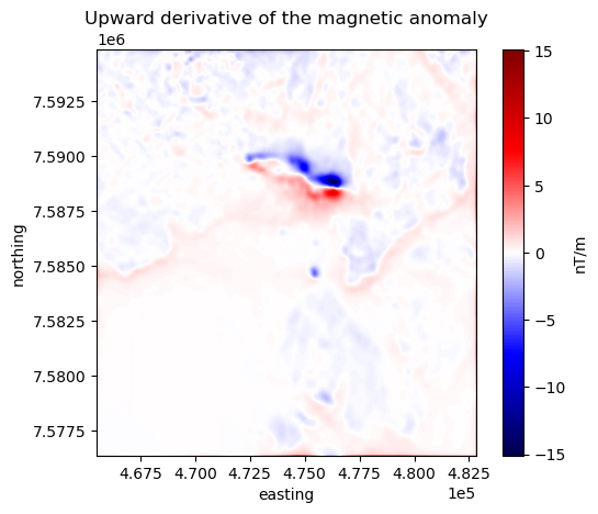
Upward derivative#
Let’s calculate the upward derivative (a.k.a. vertical derivative) of the
magnetic anomaly grid using the harmonica.derivative_upward function:
import harmonica as hm

deriv_upward = hm.derivative_upward(magnetic_grid_padded)
deriv_upward
<xarray.DataArray (northing: 616, easting: 576)> Size: 3MB
array([[-1.33181514e-05, -9.52547848e-06, -5.67287091e-06, ...,
        -2.43410150e-05, -2.07254007e-05, -1.70512251e-05],
       [-2.61443879e-05, -2.24106086e-05, -1.86195889e-05, ...,
        -3.70081237e-05, -3.34426463e-05, -2.98216205e-05],
       [-3.90061848e-05, -3.53298512e-05, -3.15993283e-05, ...,
        -4.97144108e-05, -4.61979657e-05, -4.26286722e-05],
       ...,
       [ 2.49528968e-05,  2.89296170e-05,  3.29751971e-05, ...,
         1.34293348e-05,  1.72033026e-05,  2.10442358e-05],
       [ 1.22299968e-05,  1.61441417e-05,  2.01240010e-05, ...,
         8.77265689e-07,  4.59710171e-06,  8.38123474e-06],
       [-5.26789593e-07,  3.32586838e-06,  7.24155673e-06, ...,
        -1.17127613e-05, -8.04558340e-06, -4.31716223e-06]])
Coordinates:
  * easting   (easting) float64 5kB 4.598e+05 4.598e+05 ... 4.885e+05 4.885e+05
* northing (northing) float64 5kB 7.57e+06 7.57e+06 ... 7.601e+06 7.601e+06This grid includes all the padding we added to the original magnetic grid, so
we better unpad it using xrft.unpad:
deriv_upward = xrft.unpad(deriv_upward, pad_width)
deriv_upward
<xarray.DataArray (northing: 370, easting: 346)> Size: 1MB
array([[-0.95819615, -0.62479717, -0.65249412, ...,  1.73446398,
         1.6766403 ,  2.72435657],
       [-0.63634012, -0.21904971, -0.23107569, ...,  0.49049566,
         0.45948428,  1.68409986],
       [-0.66359177, -0.2353631 , -0.24506233, ...,  0.51034737,
         0.49225437,  1.75482676],
       ...,
       [-3.39466133, -0.92997513, -0.84908229, ...,  0.187395  ,
         0.37947101,  1.13012071],
       [-3.28895188, -0.89679122, -0.84612101, ...,  0.15550382,
         0.36489592,  1.12153698],
       [-5.04820203, -2.9126185 , -2.80733457, ..., -0.11714694,
         0.3870613 ,  1.26040208]])
Coordinates:
  * easting   (easting) float64 3kB 4.655e+05 4.656e+05 ... 4.827e+05 4.828e+05
* northing (northing) float64 3kB 7.576e+06 7.576e+06 ... 7.595e+06 7.595e+06And plot it:
tmp = deriv_upward.plot(cmap="seismic", center=0, add_colorbar=False)
plt.gca().set_aspect("equal")
plt.title("Upward derivative of the magnetic anomaly")
plt.gca().ticklabel_format(style="sci", scilimits=(0, 0))
plt.colorbar(tmp, label="nT/m")
plt.show()
Horizontal derivatives#
We can also compute horizontal derivatives over a regular grid using the
harmonica.derivative_easting and harmonica.derivative_northing
functions.
deriv_easting = hm.derivative_easting(magnetic_grid)
deriv_easting
<xarray.DataArray 'total_field_anomaly' (northing: 370, easting: 346)> Size: 1MB
array([[ 0.024,  0.017,  0.004, ...,  0.016,  0.015,  0.016],
       [ 0.022,  0.015,  0.004, ...,  0.015,  0.015,  0.016],
       [ 0.022,  0.015,  0.003, ...,  0.015,  0.014,  0.014],
       ...,
       [-0.208, -0.22 , -0.221, ..., -0.553, -0.426, -0.352],
       [-0.19 , -0.207, -0.218, ..., -0.602, -0.47 , -0.39 ],
       [-0.168, -0.185, -0.2  , ..., -0.597, -0.472, -0.396]])
Coordinates:
  * easting   (easting) float64 3kB 4.655e+05 4.656e+05 ... 4.827e+05 4.828e+05
  * northing  (northing) float64 3kB 7.576e+06 7.576e+06 ... 7.595e+06 7.595e+06
height (northing, easting) float64 1MB 500.0 500.0 500.0 ... 500.0 500.0deriv_northing = hm.derivative_northing(magnetic_grid)
deriv_northing
<xarray.DataArray 'total_field_anomaly' (northing: 370, easting: 346)> Size: 1MB
array([[ 0.03 ,  0.028,  0.026, ..., -0.022, -0.022, -0.022],
       [ 0.021,  0.02 ,  0.019, ..., -0.022, -0.022, -0.023],
       [ 0.006,  0.005,  0.005, ..., -0.023, -0.024, -0.025],
       ...,
       [-0.002,  0.014,  0.022, ...,  0.103,  0.036, -0.015],
       [-0.04 , -0.02 , -0.005, ...,  0.106,  0.082,  0.06 ],
       [-0.066, -0.044, -0.022, ...,  0.108,  0.11 ,  0.104]])
Coordinates:
  * easting   (easting) float64 3kB 4.655e+05 4.656e+05 ... 4.827e+05 4.828e+05
  * northing  (northing) float64 3kB 7.576e+06 7.576e+06 ... 7.595e+06 7.595e+06
height (northing, easting) float64 1MB 500.0 500.0 500.0 ... 500.0 500.0And plot them:
fig, (ax1, ax2) = plt.subplots(
    nrows=1, ncols=2, sharey=True, figsize=(12, 8)
)

cbar_kwargs=dict(
    label="nT/m", orientation="horizontal", shrink=0.8, pad=0.08, aspect=42
)
kwargs = dict(center=0, cmap="seismic", cbar_kwargs=cbar_kwargs)

tmp = deriv_easting.plot(ax=ax1, **kwargs)
tmp = deriv_northing.plot(ax=ax2, **kwargs)

ax1.set_title("Easting derivative of the magnetic anomaly")
ax2.set_title("Northing derivative of the magnetic anomaly")
for ax in (ax1, ax2):
    ax.set_aspect("equal")
    ax.ticklabel_format(style="sci", scilimits=(0, 0))
plt.show()
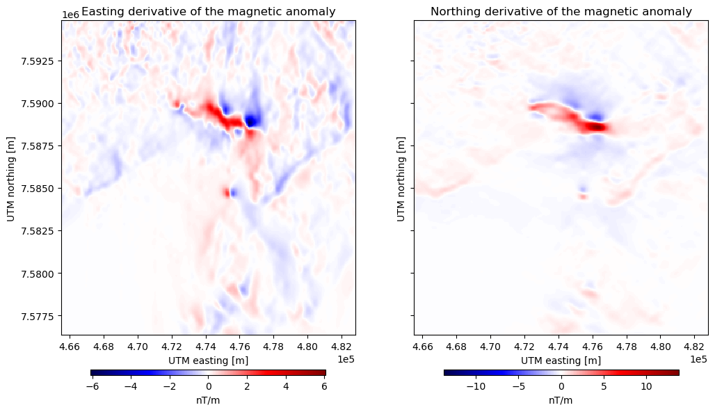
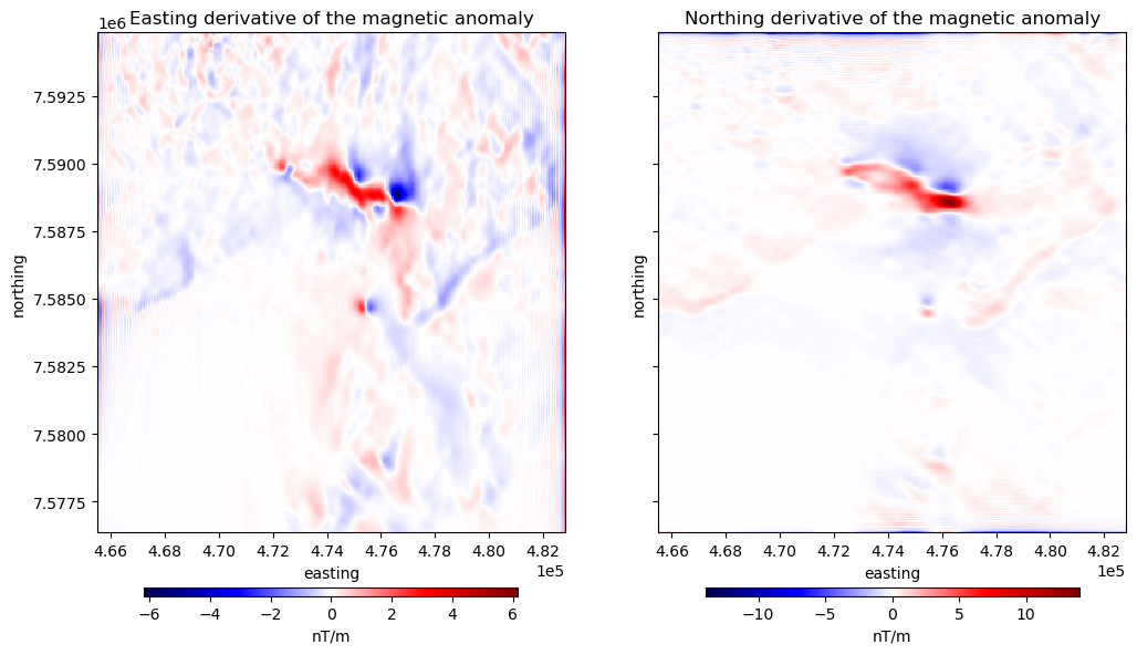
By default, these two functions compute the horizontal derivatives using
central finite differences methods. We can choose to use either the finite
difference or the FFT-based method through the method argument.
For example, we can pass method="fft" to compute the derivatives in the
frequency domain:
deriv_easting = hm.derivative_easting(magnetic_grid_padded, method="fft")
deriv_easting = xrft.unpad(deriv_easting, pad_width)
deriv_easting
<xarray.DataArray (northing: 370, easting: 346)> Size: 1MB
array([[ 0.50048199, -0.19278044,  0.13577175, ...,  0.39878843,
        -0.59429549,  1.39003591],
       [ 0.52115484, -0.20585468,  0.14315899, ...,  0.40289984,
        -0.60133441,  1.40562168],
       [ 0.52891822, -0.2086157 ,  0.14348528, ...,  0.40827692,
        -0.61014988,  1.42089306],
       ...,
       [ 2.43620373, -1.38416908,  0.49946553, ..., -0.3666967 ,
        -0.73927385,  0.42750644],
       [ 2.43711512, -1.36261715,  0.49770439, ..., -0.41819735,
        -0.78503278,  0.39910955],
       [ 2.40158711, -1.31498061,  0.50162999, ..., -0.43062165,
        -0.75785869,  0.32352971]])
Coordinates:
  * easting   (easting) float64 3kB 4.655e+05 4.656e+05 ... 4.827e+05 4.828e+05
* northing (northing) float64 3kB 7.576e+06 7.576e+06 ... 7.595e+06 7.595e+06deriv_northing = hm.derivative_northing(magnetic_grid_padded, method="fft")
deriv_northing = xrft.unpad(deriv_northing, pad_width)
deriv_northing
<xarray.DataArray (northing: 370, easting: 346)> Size: 1MB
array([[ 0.49981797,  0.51505152,  0.52085958, ..., -1.41297184,
        -1.40373407, -1.39047857],
       [-0.18344079, -0.19204679, -0.19683759, ...,  0.59467933,
         0.5912331 ,  0.58320314],
       [ 0.1326666 ,  0.13715404,  0.14021738, ..., -0.41085833,
        -0.41006472, -0.40635804],
       ...,
       [-0.67325073, -0.62931925, -0.587516  , ...,  0.04336853,
         0.07440956,  0.09627221],
       [ 1.03876541,  1.01294743,  0.97022434, ...,  0.19944866,
         0.01274978, -0.12811109],
       [-2.51808837, -2.39082378, -2.23712997, ..., -0.10561023,
         0.28247463,  0.55809873]])
Coordinates:
  * easting   (easting) float64 3kB 4.655e+05 4.656e+05 ... 4.827e+05 4.828e+05
* northing (northing) float64 3kB 7.576e+06 7.576e+06 ... 7.595e+06 7.595e+06fig, (ax1, ax2) = plt.subplots(
nrows=1, ncols=2, sharey=True, figsize=(12, 8)
)
cbar_kwargs=dict(
label="nT/m", orientation="horizontal", shrink=0.8, pad=0.08, aspect=42
)
kwargs = dict(center=0, cmap="seismic", cbar_kwargs=cbar_kwargs)
tmp = deriv_easting.plot(ax=ax1, **kwargs)
tmp = deriv_northing.plot(ax=ax2, **kwargs)
ax1.set_title("Easting derivative of the magnetic anomaly")
ax2.set_title("Northing derivative of the magnetic anomaly")
for ax in (ax1, ax2):
ax.set_aspect("equal")
ax.ticklabel_format(style="sci", scilimits=(0, 0))
plt.show()
Important
Horizontal derivatives through finite differences are usually more accurate and have less artifacts than their FFT-based counterpart.
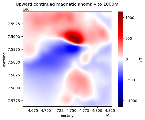
Upward continuation#
We can also upward continue the original magnetic grid. This is, estimating the magnetic field generated by the same sources at a higher altitude. The original magnetic anomaly grid is located at 500 m above the ellipsoid, as we can see in its height coordinate. If we want to get the magnetic anomaly at 1000m above the ellipsoid, we need to upward continue it a height displacement of 500m:
upward_continued = hm.upward_continuation(
    magnetic_grid_padded, height_displacement=500
)
This grid includes all the padding we added to the original magnetic grid, so
we better unpad it using xrft.unpad:
upward_continued = xrft.unpad(upward_continued, pad_width)
upward_continued
<xarray.DataArray (northing: 370, easting: 346)> Size: 1MB
array([[  1.53187928,   1.85099564,   2.13678808, ..., -33.6048979 ,
        -31.65891672, -29.67750887],
       [  1.82032573,   2.17483923,   2.49235855, ..., -35.9639625 ,
        -33.83599574, -31.66680075],
       [  2.07316733,   2.45926837,   2.80498407, ..., -38.27996857,
        -35.97492957, -33.62308159],
       ...,
       [ 50.44855928,  53.84377734,  57.13891805, ...,   4.05301094,
          2.81272119,   1.76442772],
       [ 47.56513259,  50.69950849,  53.74613485, ...,   4.6684348 ,
          3.44419849,   2.39520294],
       [ 44.63682346,  47.50470212,  50.29751413, ...,   5.03755398,
          3.86191533,   2.84250143]])
Coordinates:
  * easting   (easting) float64 3kB 4.655e+05 4.656e+05 ... 4.827e+05 4.828e+05
* northing (northing) float64 3kB 7.576e+06 7.576e+06 ... 7.595e+06 7.595e+06And plot it:
tmp = upward_continued.plot(cmap="seismic", center=0, add_colorbar=False)
plt.gca().set_aspect("equal")
plt.title("Upward continued magnetic anomaly to 1000m")
plt.gca().ticklabel_format(style="sci", scilimits=(0, 0))
plt.colorbar(tmp, label="nT")
plt.show()
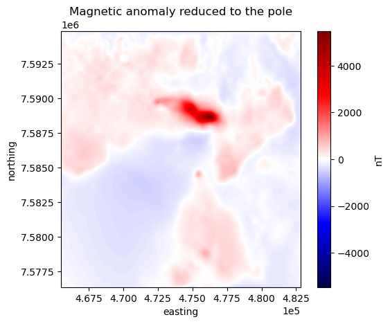
Reduction to the pole#
We can also apply a reduction to the pole to any magnetic anomaly grid.
This transformation consists in obtaining the magnetic anomaly of the same
sources as if they were located on the North magnetic pole.
We can apply it through the harmonica.reduction_to_pole function.
Important
Applying reduction to the pole to low latitude regions can amplify high frequency noise.
The reduction to the pole needs information about the orientation of the geomagnetic field at the location of the survey and also the orientation of the magnetization vector of the sources.
The International Global Reference Field (IGRF) can provide us information about the inclination and declination of the geomagnetic field at the time of the survey (1990 in this case):
inclination, declination = -52.98, 6.51
If we consider that the sources are magnetized in the same direction as the
geomagnetic survey (hypothesis that is true in case the sources don’t have any
remanence), then we can apply the reduction to the pole passing only the
inclination and declination of the geomagnetic field:
rtp_grid = hm.reduction_to_pole(
    magnetic_grid_padded, inclination=inclination, declination=declination
)

# Unpad the reduced to the pole grid
rtp_grid = xrft.unpad(rtp_grid, pad_width)
rtp_grid
<xarray.DataArray (northing: 370, easting: 346)> Size: 1MB
array([[  14.15546834,   10.38425778,   10.01995891, ..., -219.8102288 ,
        -210.9302948 , -179.38411068],
       [  -3.21249403,   -9.37124449,  -10.96593068, ..., -165.15297526,
        -158.09589683, -133.29346492],
       [  -2.32174677,   -9.44940979,  -11.35233997, ..., -170.79739203,
        -165.2567305 , -141.04626566],
       ...,
       [  45.45701952,  -24.80999268,  -51.27393509, ...,  -40.42602057,
         -64.12371145,  -75.97556295],
       [  36.9104954 ,  -37.13717695,  -58.40650833, ...,  -34.55584156,
         -55.6561726 ,  -71.01718702],
       [-102.42450988, -155.67867833, -165.96638688, ...,  -36.95818214,
         -35.0401052 ,  -40.15055123]])
Coordinates:
  * easting   (easting) float64 3kB 4.655e+05 4.656e+05 ... 4.827e+05 4.828e+05
* northing (northing) float64 3kB 7.576e+06 7.576e+06 ... 7.595e+06 7.595e+06And plot it:
tmp = rtp_grid.plot(cmap="seismic", center=0, add_colorbar=False)
plt.gca().set_aspect("equal")
plt.title("Magnetic anomaly reduced to the pole")
plt.gca().ticklabel_format(style="sci", scilimits=(0, 0))
plt.colorbar(tmp, label="nT")
plt.show()
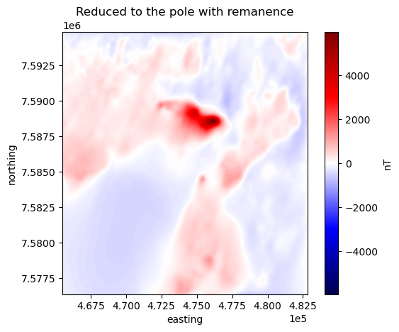
If on the other hand we have any knowledge about the orientation of the
magnetization vector of the sources, we can specify the
magnetization_inclination and magnetization_declination:
mag_inclination, mag_declination = -25, 21

tmp = rtp_grid = hm.reduction_to_pole(
    magnetic_grid_padded,
    inclination=inclination,
    declination=declination,
    magnetization_inclination=mag_inclination,
    magnetization_declination=mag_declination,
)

# Unpad the reduced to the pole grid
rtp_grid = xrft.unpad(rtp_grid, pad_width)
rtp_grid
<xarray.DataArray (northing: 370, easting: 346)> Size: 1MB
array([[ -77.45230222, -114.40589805, -117.03964335, ...,  -87.74331941,
         -75.65311441,   43.0543142 ],
       [ -99.41773744, -137.48348629, -141.5147968 , ...,  -31.30662147,
         -20.40281657,   92.22748918],
       [ -99.90966143, -139.38038808, -143.11784398, ...,  -38.52922255,
         -29.73746893,   83.23553188],
       ...,
       [  13.25374634, -170.27669068, -163.93668068, ...,  -44.43378324,
         -80.78993325,  -66.8060264 ],
       [ -28.47757862, -187.01875868, -173.90317006, ...,  -27.82016979,
         -55.31902009,  -61.09794208],
       [-236.07958913, -301.62729697, -299.61024736, ...,  -28.01930179,
         -18.38082429,  -22.65814366]])
Coordinates:
  * easting   (easting) float64 3kB 4.655e+05 4.656e+05 ... 4.827e+05 4.828e+05
* northing (northing) float64 3kB 7.576e+06 7.576e+06 ... 7.595e+06 7.595e+06tmp = rtp_grid.plot(cmap="seismic", center=0, add_colorbar=False)
plt.gca().set_aspect("equal")
plt.title("Reduced to the pole with remanence")
plt.gca().ticklabel_format(style="sci", scilimits=(0, 0))
plt.colorbar(tmp, label="nT")
plt.show()
Gaussian filters#
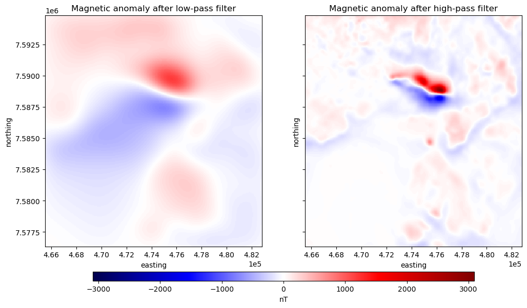
We can also apply Gaussian low-pass and high-pass filters to any regular grid.
These two need us to select a cutoff wavelength.
The low-pass filter will remove any signal with a high spatial frequency,
keeping only the signal components that have a wavelength higher than the
selected cutoff wavelength.
The high-pass filter, on the other hand, removes any signal with a low spatial
frequency, keeping only the components with a wavelength lower than the cutoff
wavelength.
These two filters can be applied to our regular grid with the
harmonica.gaussian_lowpass and harmonica.gaussian_highpass.
Let’s define a cutoff wavelength of 5 kilometers:
cutoff_wavelength = 5e3
Then apply the two filters to our padded magnetic grid:
magnetic_low_freqs = hm.gaussian_lowpass(
    magnetic_grid_padded, wavelength=cutoff_wavelength
)
magnetic_high_freqs = hm.gaussian_highpass(
    magnetic_grid_padded, wavelength=cutoff_wavelength
)
And unpad them:
magnetic_low_freqs = xrft.unpad(magnetic_low_freqs, pad_width)
magnetic_high_freqs = xrft.unpad(magnetic_high_freqs, pad_width)
magnetic_low_freqs
<xarray.DataArray (northing: 370, easting: 346)> Size: 1MB
array([[ 4.60585742e+00,  4.72025807e+00,  4.81814332e+00, ...,
        -3.68551963e+01, -3.50940549e+01, -3.33406590e+01],
       [ 4.70587584e+00,  4.81991561e+00,  4.91668718e+00, ...,
        -3.87398587e+01, -3.68891989e+01, -3.50465543e+01],
       [ 4.78689168e+00,  4.89969232e+00,  4.99448397e+00, ...,
        -4.06231237e+01, -3.86830315e+01, -3.67512125e+01],
       ...,
       [ 5.24052307e+01,  5.51977692e+01,  5.80158045e+01, ...,
        -8.46624027e-01, -1.00254650e+00, -1.16000669e+00],
       [ 5.00637788e+01,  5.27307718e+01,  5.54221609e+01, ...,
         1.79766185e-01, -1.44140930e-02, -2.10519096e-01],
       [ 4.77049435e+01,  5.02456818e+01,  5.28097178e+01, ...,
         1.08696676e+00,  8.60201189e-01,  6.31169136e-01]])
Coordinates:
  * easting   (easting) float64 3kB 4.655e+05 4.656e+05 ... 4.827e+05 4.828e+05
* northing (northing) float64 3kB 7.576e+06 7.576e+06 ... 7.595e+06 7.595e+06magnetic_high_freqs
<xarray.DataArray (northing: 370, easting: 346)> Size: 1MB
array([[ 30.39409376,  31.4796931 ,  31.88180785, ..., -64.24485251,
        -65.3059939 , -66.25938981],
       [ 31.79407534,  32.78003556,  33.08326399, ..., -63.46019009,
        -64.6108499 , -65.65349454],
       [ 32.3130595 ,  33.30025885,  33.6054672 , ..., -62.6769251 ,
        -63.91701728, -65.14883631],
       ...,
       [130.3947205 , 117.20218197, 102.78414668, ...,   1.6465752 ,
        -23.19750233, -40.64004214],
       [132.03617232, 119.86917935, 105.97779024, ...,   5.82018499,
        -21.48563474, -40.78952973],
       [131.09500767, 120.15426938, 107.49023338, ...,  10.31298441,
        -16.86025002, -36.43121796]])
Coordinates:
  * easting   (easting) float64 3kB 4.655e+05 4.656e+05 ... 4.827e+05 4.828e+05
* northing (northing) float64 3kB 7.576e+06 7.576e+06 ... 7.595e+06 7.595e+06Let’s plot the results side by side:
import verde as vd

fig, (ax1, ax2) = plt.subplots(
    nrows=1, ncols=2, sharey=True, figsize=(12, 8)
)

maxabs = vd.maxabs(magnetic_low_freqs, magnetic_high_freqs)
kwargs = dict(cmap="seismic", vmin=-maxabs, vmax=maxabs, add_colorbar=False)

tmp = magnetic_low_freqs.plot(ax=ax1, **kwargs)
tmp = magnetic_high_freqs.plot(ax=ax2, **kwargs)

ax1.set_title("Magnetic anomaly after low-pass filter")
ax2.set_title("Magnetic anomaly after high-pass filter")
for ax in (ax1, ax2):
    ax.set_aspect("equal")
    ax.ticklabel_format(style="sci", scilimits=(0, 0))

plt.colorbar(
    tmp,
    ax=[ax1, ax2],
    label="nT",
    orientation="horizontal",
    aspect=42,
    shrink=0.8,
    pad=0.08,
)
plt.show()
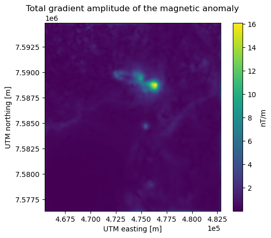
Total gradient amplitude#
Hint
Total gradient amplitude is also known as analytic signal.
We can also calculate the total gradient amplitude of any magnetic anomaly grid. This transformation consists in obtaining the amplitude of the gradient of the magnetic field in all the three spatial directions by applying
We can apply it through the harmonica.total_gradient_amplitude function.
tga_grid = hm.total_gradient_amplitude(
    magnetic_grid_padded
)

# Unpad the total gradient amplitude grid
tga_grid = xrft.unpad(tga_grid, pad_width)
tga_grid
<xarray.DataArray (northing: 370, easting: 346)> Size: 1MB
array([[1.08738592, 0.72940807, 0.75509218, ..., 2.0132328 , 1.95999329,
        3.07313939],
       [0.73942233, 0.22047172, 0.23189001, ..., 0.49121787, 0.46025515,
        1.96645552],
       [0.76571121, 0.23589359, 0.24513169, ..., 0.51108555, 0.49303789,
        2.03290899],
       ...,
       [3.80734867, 0.95574565, 0.87764784, ..., 0.59290377, 0.57163822,
        1.15583825],
       [3.71454961, 0.92058867, 0.87376757, ..., 0.63073088, 0.60064385,
        1.14353417],
       [5.63063027, 3.39067041, 3.24439853, ..., 0.61133653, 0.64716741,
        1.33503332]])
Coordinates:
  * easting   (easting) float64 3kB 4.655e+05 4.656e+05 ... 4.827e+05 4.828e+05
* northing (northing) float64 3kB 7.576e+06 7.576e+06 ... 7.595e+06 7.595e+06And plot it:
import verde as vd

tmp = tga_grid.plot(cmap="viridis", add_colorbar=False)
plt.gca().set_aspect("equal")
plt.title("Total gradient amplitude of the magnetic anomaly")
plt.gca().ticklabel_format(style="sci", scilimits=(0, 0))
plt.colorbar(tmp, label="nT/m")
plt.show()