Gradient-boosted equivalent sources#
As mentioned in Equivalent Sources, one of the main drawbacks of the
equivalent sources technique is the high computational load required to
estimate source coefficients and ultimately to predict field values.
During the source coefficients estimation step (while running the
harmonica.EquivalentSources.fit method) a Jacobian matrix with a size
of number of sources times number of observation points must be built.
This Jacobian matrix could become too large to fit in memory if the number of
data points and sources are too big.
Note
Interpolating 200000 data points using 200000 sources would require more than 300 GB only to store the Jacobian matrix (using 64 bits floats for each matrix element).
One way to reduce the memory requirement is using Block-averaged equivalent sources, but it might be not enough when working with very large datasets.
A solution to this problem is to use gradient-boosted equivalent sources, introduced in [Soler2021]. This new methodology creates \(k\) overlapping windows of equal size that cover the entire survey area and defines one set of equivalent sources for each windows, where each set is formed by the original equivalent sources that fall inside its corresponding window. The estimation of the coefficients is then carried out iteratively passing through one window at a time. On each iteration the coefficients of the selected subset of sources are fit against the observation points that fall inside the same window. After each iteration the field generated by those adjusted sources are predicted on every computation point and the residue is updated. The process finishes when every window has been visited.
The gradient-boosted equivalent sources have been included in Harmonica and can
be used through the harmonica.EquivalentSourcesGB class.
Lets load some gravity data for Southern Africa:
import ensaio
import pandas as pd

fname = ensaio.fetch_southern_africa_gravity(version=1)
data = pd.read_csv(fname)
data
| longitude | latitude | height_sea_level_m | gravity_mgal | |
|---|---|---|---|---|
| 0 | 18.34444 | -34.12971 | 32.2 | 979656.12 |
| 1 | 18.36028 | -34.08833 | 592.5 | 979508.21 |
| 2 | 18.37418 | -34.19583 | 18.4 | 979666.46 |
| 3 | 18.40388 | -34.23972 | 25.0 | 979671.03 |
| 4 | 18.41112 | -34.16444 | 228.7 | 979616.11 |
| ... | ... | ... | ... | ... |
| 14354 | 21.22500 | -17.95833 | 1053.1 | 978182.09 |
| 14355 | 21.27500 | -17.98333 | 1033.3 | 978183.09 |
| 14356 | 21.70833 | -17.99166 | 1041.8 | 978182.69 |
| 14357 | 21.85000 | -17.95833 | 1033.3 | 978193.18 |
| 14358 | 21.98333 | -17.94166 | 1022.6 | 978211.38 |
14359 rows × 4 columns
Note
This gravity dataset is small enough to be interpolated with equivalent sources in any modest personal computer. Nevertheless, we will grid it using gradient-boosted equivalent sources to speed up the computations on this small example.
Compute gravity disturbance by subtracting normal gravity using boule
(see Gravity Disturbance for more information):
import boule as bl

normal_gravity = bl.WGS84.normal_gravity(data.latitude, data.height_sea_level_m)
disturbance = data.gravity_mgal - normal_gravity
And project the data to plain coordinates using a Mercator projection:
import pyproj

projection = pyproj.Proj(proj="merc", lat_ts=data.latitude.mean())
easting, northing = projection(data.longitude.values, data.latitude.values)
coordinates = (easting, northing, data.height_sea_level_m)
We can define some gradient-boosted equivalent sources through the
harmonica.EquivalentSourcesGB. When doing so we need to specify the
size of the windows that will be used in the gradient boosting process.
We will use square windows of 100 km per side.
Moreover, gradient-boosted equivalent sources can be used together with
Block-averaged equivalent sources. We will do so choosing a block size of 2 km
per side.
import harmonica as hm

eqs = hm.EquivalentSourcesGB(
    depth=9e3, damping=10, block_size=2e3, window_size=100e3, random_state=42
)
Important
Smaller windows reduce the memory requirements for building the Jacobian matrix, but also reduces the accuracy of the interpolations. We recommend using the maximum window size that produces Jacobian matrices that can fit in memory.
Note
The order in which windows are explored is randomized. By passing a value
to random_state we ensure to obtain always the same result everytime we
fit these equivalent sources.
We can use the harmonica.EquivalentSourcesGB.estimate_required_memory
method to find out how much memory we will need to store the Jacobian matrix
given the coordinates of the observation points. The value is given in bytes.
eqs.estimate_required_memory(coordinates)
np.int64(1210568)
Once we are sure that we have enough memory to store these Jacobian matrices we can fit the sources against the gravity disturbance data:
eqs.fit(coordinates, disturbance)
EquivalentSourcesGB(block_size=2000.0, damping=10, depth=9000.0,
                    random_state=42, window_size=100000.0)
In a Jupyter environment, please rerun this cell to show the HTML representation or trust the notebook. On GitHub, the HTML representation is unable to render, please try loading this page with nbviewer.org.
EquivalentSourcesGB(block_size=2000.0, damping=10, depth=9000.0,
                    random_state=42, window_size=100000.0)
And then predict the field on a regular grid of computation points:
import verde as vd
region = vd.get_region(coordinates)
grid_coords = vd.grid_coordinates(
    region=region,
    spacing=5e3,
    extra_coords=2.5e3,
)
grid = eqs.grid(grid_coords, data_names=["gravity_disturbance"])
grid
<xarray.Dataset> Size: 3MB
Dimensions:              (northing: 389, easting: 412)
Coordinates:
  * easting              (easting) float64 3kB 1.174e+06 1.179e+06 ... 3.228e+06
  * northing             (northing) float64 3kB -3.665e+06 ... -1.724e+06
    upward               (northing, easting) float64 1MB 2.5e+03 ... 2.5e+03
Data variables:
    gravity_disturbance  (northing, easting) float64 1MB 5.88 5.895 ... 4.188
Attributes:
metadata: Generated by EquivalentSourcesGB(block_size=2000.0, damping=10...Since this particular dataset doesn’t have a good coverage of the entire area,
we might want to mask the output grid based on the distance to the closest data
point. We can do so through the verde.distance_mask function.
grid_masked = vd.distance_mask(coordinates, maxdist=50e3, grid=grid)
And plot it:
import pygmt
# Set figure properties
w, e, s, n = region
fig_height = 10
fig_width = fig_height * (e - w) / (n - s)
fig_ratio = (n - s) / (fig_height / 100)
fig_proj = f"x1:{fig_ratio}"
maxabs = vd.maxabs(disturbance, grid_masked.gravity_disturbance)
fig = pygmt.Figure()
# Make colormap of data
pygmt.makecpt(cmap="polar+h0",series=(-maxabs, maxabs,))
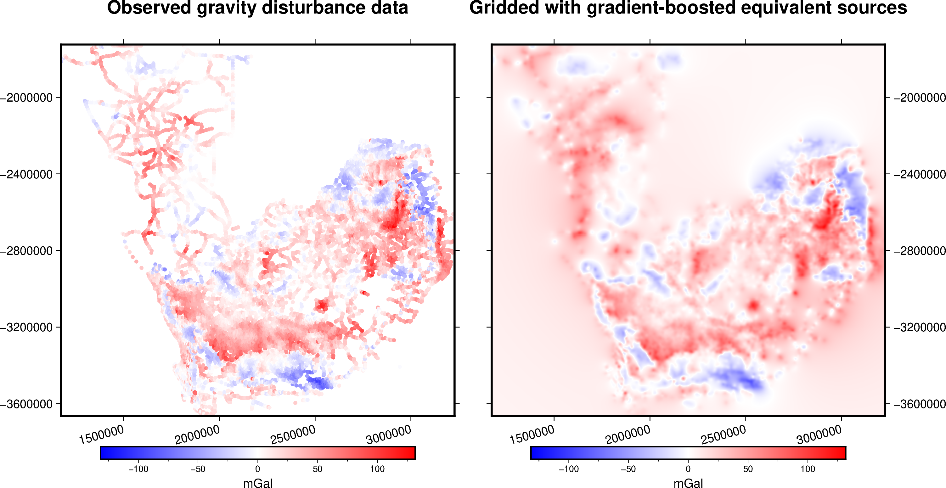
title = "Observed gravity disturbance data"
with pygmt.config(FONT_TITLE="14p"):
fig.plot(
projection=fig_proj,
region=region,
frame=[f"WSne+t{title}", "xa500000+a15", "ya400000"],
x=easting,
y=northing,
fill=disturbance,
style="c0.1c",
cmap=True,
)
fig.colorbar(cmap=True, frame=["a50f25", "x+lmGal"])
fig.shift_origin(xshift=fig_width + 1)
title = "Gridded with gradient-boosted equivalent sources"
with pygmt.config(FONT_TITLE="14p"):
fig.grdimage(
frame=[f"ESnw+t{title}", "xa500000+a15", "ya400000"],
grid=grid.gravity_disturbance,
cmap=True,
)
fig.colorbar(cmap=True, frame=["a50f25", "x+lmGal"])
fig.show()