Using Weights

One of the advantages of using a Green’s functions approach to interpolation is that we can easily weight the data to give each point more or less influence over the results. This is a good way to not let data points with large uncertainties bias the interpolation or the data decimation.

import cartopy.crs as ccrs
import matplotlib.pyplot as plt
import numpy as np
import pyproj

# The weights vary a lot so it's better to plot them using a logarithmic color
# scale
from matplotlib.colors import LogNorm

import verde as vd

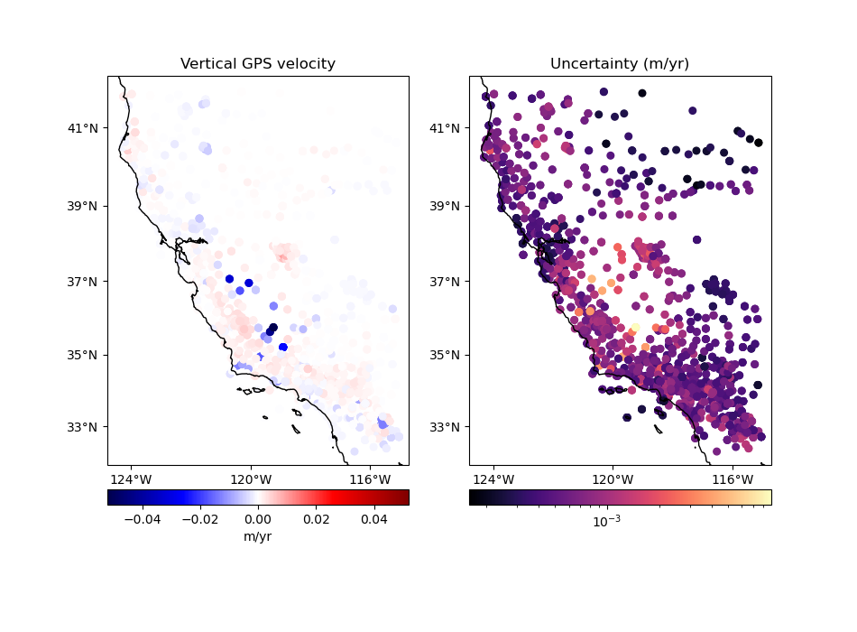
We’ll use some sample GPS vertical ground velocity which has some variable uncertainties associated with each data point. The data are loaded as a pandas.DataFrame:

data = vd.datasets.fetch_california_gps()
print(data.head())

    latitude   longitude     height  ...  std_north  std_east   std_up
0  34.116409  242.906804  762.11978  ...     0.0002   0.00037  0.00053
1  34.116409  242.906804  762.10883  ...     0.0002   0.00037  0.00053
2  34.116409  242.906805  762.09364  ...     0.0002   0.00037  0.00053
3  34.116409  242.906805  762.09073  ...     0.0002   0.00037  0.00053
4  34.116409  242.906805  762.07699  ...     0.0002   0.00037  0.00053

[5 rows x 9 columns]

Let’s plot our data using Cartopy to see what the vertical velocities and their uncertainties look like. We’ll make a function for this so we can reuse it later on.

def plot_data(coordinates, velocity, weights, title_data, title_weights):
    "Make two maps of our data, one with the data and one with the weights"
    fig, axes = plt.subplots(
        1, 2, figsize=(9.5, 7), subplot_kw=dict(projection=ccrs.Mercator())
    )
    crs = ccrs.PlateCarree()
    ax = axes[0]
    ax.set_title(title_data)
    maxabs = vd.maxabs(velocity)
    pc = ax.scatter(
        *coordinates,
        c=velocity,
        s=30,
        cmap="seismic",
        vmin=-maxabs,
        vmax=maxabs,
        transform=crs,
    )
    plt.colorbar(pc, ax=ax, orientation="horizontal", pad=0.05).set_label("m/yr")
    vd.datasets.setup_california_gps_map(ax)
    ax = axes[1]
    ax.set_title(title_weights)
    pc = ax.scatter(
        *coordinates, c=weights, s=30, cmap="magma", transform=crs, norm=LogNorm()
    )
    plt.colorbar(pc, ax=ax, orientation="horizontal", pad=0.05)
    vd.datasets.setup_california_gps_map(ax)
    plt.show()


# Plot the data and the uncertainties
plot_data(
    (data.longitude, data.latitude),
    data.velocity_up,
    data.std_up,
    "Vertical GPS velocity",
    "Uncertainty (m/yr)",
)

Weights in data decimation

BlockReduce can’t output weights for each data point because it doesn’t know which reduction operation it’s using. If you want to do a weighted interpolation, like verde.Spline, BlockReduce won’t propagate the weights to the interpolation function. If your data are relatively smooth, you can use verde.BlockMean instead to decimated data and produce weights. It can calculate different kinds of weights, depending on configuration options and what you give it as input.

Let’s explore all of the possibilities.

mean = vd.BlockMean(spacing=15 / 60)
print(mean)

BlockMean(spacing=0.25)

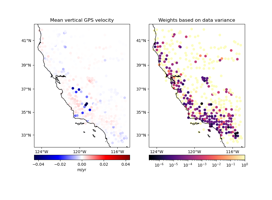
Option 1: No input weights

In this case, we’ll get a standard mean and the output weights will be 1 over the variance of the data in each block:

\[\bar{d} = \dfrac{\sum\limits_{i=1}^N d_i}{N} \: , \qquad \sigma^2 = \dfrac{\sum\limits_{i=1}^N (d_i - \bar{d})^2}{N} \: , \qquad w = \dfrac{1}{\sigma^2}\]

in which \(N\) is the number of data points in the block, \(d_i\) are the data values in the block, and the output values for the block are the mean data \(\bar{d}\) and the weight \(w\).

Notice that data points that are more uncertain don’t necessarily have smaller weights. Instead, the blocks that contain data with sharper variations end up having smaller weights, like the data points in the south.

coordinates, velocity, weights = mean.filter(
    coordinates=(data.longitude, data.latitude), data=data.velocity_up
)

plot_data(
    coordinates,
    velocity,
    weights,
    "Mean vertical GPS velocity",
    "Weights based on data variance",
)

/usr/share/miniconda/envs/test/lib/python3.12/site-packages/verde/blockreduce.py:469: FutureWarning: The provided callable <function var at 0x7fd602476e80> is currently using SeriesGroupBy.var. In a future version of pandas, the provided callable will be used directly. To keep current behavior pass the string "var" instead.
  blocked = table.groupby("block").aggregate(reduction)

Option 2: Input weights are not related to the uncertainty of the data

This is the case when data weights are chosen by the user, not based on the measurement uncertainty. For example, when you need to give less importance to a portion of the data and no uncertainties are available. The mean will be weighted and the output weights will be 1 over the weighted variance of the data in each block:

\[\bar{d}^* = \dfrac{\sum\limits_{i=1}^N w_i d_i}{\sum\limits_{i=1}^N w_i} \: , \qquad \sigma^2_w = \dfrac{\sum\limits_{i=1}^N w_i(d_i - \bar{d}*)^2}{ \sum\limits_{i=1}^N w_i} \: , \qquad w = \dfrac{1}{\sigma^2_w}\]

in which \(w_i\) are the input weights in the block.

The output will be similar to the one above but points with larger initial weights will have a smaller influence on the mean and also on the output weights.

# We'll use 1 over the squared data uncertainty as our input weights.
data["weights"] = 1 / data.std_up**2

# By default, BlockMean assumes that weights are not related to uncertainties
coordinates, velocity, weights = mean.filter(
    coordinates=(data.longitude, data.latitude),
    data=data.velocity_up,
    weights=data.weights,
)

plot_data(
    coordinates,
    velocity,
    weights,
    "Weighted mean vertical GPS velocity",
    "Weights based on weighted data variance",
)

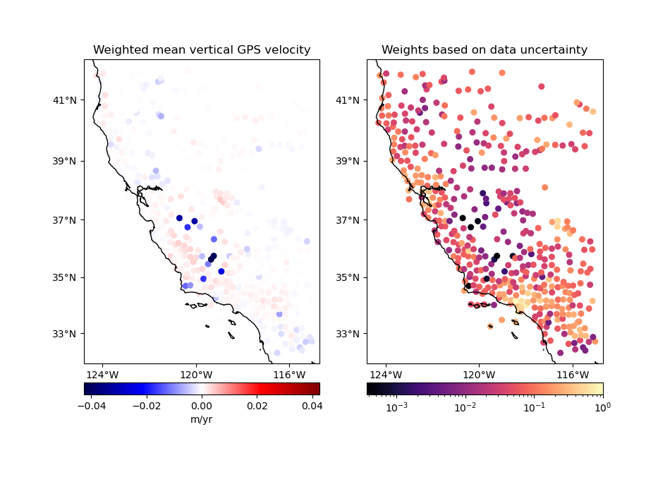
Option 3: Input weights are 1 over the data uncertainty squared

If input weights are 1 over the data uncertainty squared, we can use uncertainty propagation to calculate the uncertainty of the weighted mean and use it to define our output weights. Use option uncertainty=True to tell BlockMean to calculate weights based on the propagated uncertainty of the data. The output weights will be 1 over the propagated uncertainty squared. In this case, the input weights must not be normalized. This is preferable if you know the uncertainty of the data.

\[w_i = \dfrac{1}{\sigma_i^2} \: , \qquad \sigma_{\bar{d}^*}^2 = \dfrac{1}{\sum\limits_{i=1}^N w_i} \: , \qquad w = \dfrac{1}{\sigma_{\bar{d}^*}^2}\]

in which \(\sigma_i\) are the input data uncertainties in the block and \(\sigma_{\bar{d}^*}\) is the propagated uncertainty of the weighted mean in the block.

Notice that in this case the output weights reflect the input data uncertainties. Less weight is given to the data points that had larger uncertainties from the start.

# Configure BlockMean to assume that the input weights are 1/uncertainty**2
mean = vd.BlockMean(spacing=15 / 60, uncertainty=True)

coordinates, velocity, weights = mean.filter(
    coordinates=(data.longitude, data.latitude),
    data=data.velocity_up,
    weights=data.weights,
)

plot_data(
    coordinates,
    velocity,
    weights,
    "Weighted mean vertical GPS velocity",
    "Weights based on data uncertainty",
)

Note

Output weights are always normalized to the ]0, 1] range. See verde.variance_to_weights.

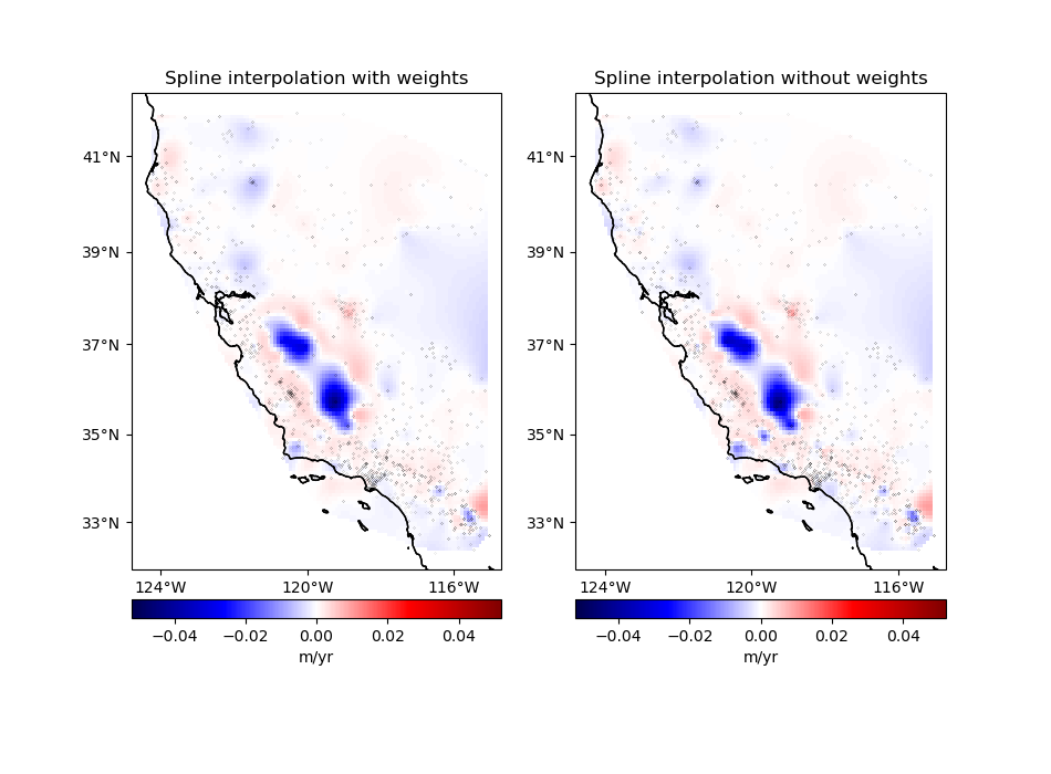
Interpolation with weights

The Green’s functions based interpolation classes in Verde, like Spline, can take input weights if you want to give less importance to some data points. In our case, the points with larger uncertainties shouldn’t have the same influence in our gridded solution as the points with lower uncertainties.

Let’s setup a projection to grid our geographic data using the Cartesian spline gridder.

projection = pyproj.Proj(proj="merc", lat_ts=data.latitude.mean())
proj_coords = projection(data.longitude.values, data.latitude.values)

region = vd.get_region(coordinates)
spacing = 5 / 60

Now we can grid our data using a weighted spline. We’ll use the block mean results with uncertainty based weights.

Note that the weighted spline solution will only work on a non-exact interpolation. So we’ll need to use some damping regularization or not use the data locations for the point forces. Here, we’ll apply a bit of damping.

spline = vd.Chain(
    [
        # Convert the spacing to meters because Spline is a Cartesian gridder
        ("mean", vd.BlockMean(spacing=spacing * 111e3, uncertainty=True)),
        ("spline", vd.Spline(damping=1e-10)),
    ]
).fit(proj_coords, data.velocity_up, data.weights)
grid = spline.grid(
    region=region,
    spacing=spacing,
    projection=projection,
    dims=["latitude", "longitude"],
    data_names="velocity",
)
# Avoid showing interpolation outside of the convex hull of the data points.
grid = vd.convexhull_mask(coordinates, grid=grid, projection=projection)

Calculate an unweighted spline as well for comparison.

spline_unweighted = vd.Chain(
    [
        ("mean", vd.BlockReduce(np.mean, spacing=spacing * 111e3)),
        ("spline", vd.Spline()),
    ]
).fit(proj_coords, data.velocity_up)
grid_unweighted = spline_unweighted.grid(
    region=region,
    spacing=spacing,
    projection=projection,
    dims=["latitude", "longitude"],
    data_names="velocity",
)
grid_unweighted = vd.convexhull_mask(
    coordinates, grid=grid_unweighted, projection=projection
)

/usr/share/miniconda/envs/test/lib/python3.12/site-packages/verde/blockreduce.py:179: FutureWarning: The provided callable <function mean at 0x7fd602476c00> is currently using DataFrameGroupBy.mean. In a future version of pandas, the provided callable will be used directly. To keep current behavior pass the string "mean" instead.
  blocked = pd.DataFrame(columns).groupby("block").aggregate(reduction)
/usr/share/miniconda/envs/test/lib/python3.12/site-packages/verde/blockreduce.py:236: FutureWarning: The provided callable <function mean at 0x7fd602476c00> is currently using DataFrameGroupBy.mean. In a future version of pandas, the provided callable will be used directly. To keep current behavior pass the string "mean" instead.
  grouped = table.groupby("block").aggregate(self.reduction)

Finally, plot the weighted and unweighted grids side by side.

fig, axes = plt.subplots(
    1, 2, figsize=(9.5, 7), subplot_kw=dict(projection=ccrs.Mercator())
)
crs = ccrs.PlateCarree()
ax = axes[0]
ax.set_title("Spline interpolation with weights")
maxabs = vd.maxabs(data.velocity_up)
pc = grid.velocity.plot.pcolormesh(
    ax=ax,
    cmap="seismic",
    vmin=-maxabs,
    vmax=maxabs,
    transform=crs,
    add_colorbar=False,
    add_labels=False,
)
plt.colorbar(pc, ax=ax, orientation="horizontal", pad=0.05).set_label("m/yr")
ax.plot(data.longitude, data.latitude, ".k", markersize=0.1, transform=crs)
ax.coastlines()
vd.datasets.setup_california_gps_map(ax)
ax = axes[1]
ax.set_title("Spline interpolation without weights")
pc = grid_unweighted.velocity.plot.pcolormesh(
    ax=ax,
    cmap="seismic",
    vmin=-maxabs,
    vmax=maxabs,
    transform=crs,
    add_colorbar=False,
    add_labels=False,
)
plt.colorbar(pc, ax=ax, orientation="horizontal", pad=0.05).set_label("m/yr")
ax.plot(data.longitude, data.latitude, ".k", markersize=0.1, transform=crs)
ax.coastlines()
vd.datasets.setup_california_gps_map(ax)
plt.show()