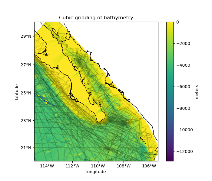
Gridding with a cubic interpolator

Verde offers the verde.Cubic class for piecewise cubic gridding. It uses scipy.interpolate.CloughTocher2DInterpolator under the hood while offering the convenience of Verde’s gridder API.

The interpolation works on Cartesian data, so if we want to grid geographic data (like our Baja California bathymetry) we need to project them into a Cartesian system. We’ll use pyproj to calculate a Mercator projection for the data.

For convenience, Verde still allows us to make geographic grids by passing the projection argument to verde.Cubic.grid and the like. When doing so, the grid will be generated using geographic coordinates which will be projected prior to interpolation.

/usr/share/miniconda/envs/test/lib/python3.12/site-packages/verde/blockreduce.py:179: FutureWarning: The provided callable <function median at 0x7fd6023a7b00> is currently using DataFrameGroupBy.median. In a future version of pandas, the provided callable will be used directly. To keep current behavior pass the string "median" instead.
  blocked = pd.DataFrame(columns).groupby("block").aggregate(reduction)
/usr/share/miniconda/envs/test/lib/python3.12/site-packages/verde/blockreduce.py:236: FutureWarning: The provided callable <function median at 0x7fd6023a7b00> is currently using DataFrameGroupBy.median. In a future version of pandas, the provided callable will be used directly. To keep current behavior pass the string "median" instead.
  grouped = table.groupby("block").aggregate(self.reduction)
Data region: (245.0, 254.705, 20.0, 29.99131)
Generated geographic grid:
<xarray.Dataset> Size: 3MB
Dimensions:       (latitude: 600, longitude: 583)
Coordinates:
  * longitude     (longitude) float64 5kB 245.0 245.0 245.0 ... 254.7 254.7
  * latitude      (latitude) float64 5kB 20.0 20.02 20.03 ... 29.96 29.97 29.99
Data variables:
    bathymetry_m  (latitude, longitude) float64 3MB nan nan nan ... nan nan nan
Attributes:
    metadata:  Generated by Cubic()

import cartopy.crs as ccrs
import matplotlib.pyplot as plt
import numpy as np
import pyproj

import verde as vd

# We'll test this on the Baja California shipborne bathymetry data
data = vd.datasets.fetch_baja_bathymetry()

# Before gridding, we need to decimate the data to avoid aliasing because of
# the oversampling along the ship tracks. We'll use a blocked median with 1
# arc-minute blocks.
spacing = 1 / 60
reducer = vd.BlockReduce(reduction=np.median, spacing=spacing)
coordinates, bathymetry = reducer.filter(
    (data.longitude, data.latitude), data.bathymetry_m
)

# Project the data using pyproj so that we can use it as input for the gridder.
# We'll set the latitude of true scale to the mean latitude of the data.
projection = pyproj.Proj(proj="merc", lat_ts=data.latitude.mean())
proj_coordinates = projection(*coordinates)

# Now we can set up a gridder for the decimated data
grd = vd.Cubic().fit(proj_coordinates, bathymetry)

# Get the grid region in geographic coordinates
region = vd.get_region((data.longitude, data.latitude))
print("Data region:", region)

# The 'grid' method can still make a geographic grid if we pass in a projection
# function that converts lon, lat into the easting, northing coordinates that
# we used in 'fit'. This can be any function that takes lon, lat and returns x,
# y. In our case, it'll be the 'projection' variable that we created above.
# We'll also set the names of the grid dimensions and the name the data
# variable in our grid (the default would be 'scalars', which isn't very
# informative).
grid = grd.grid(
    region=region,
    spacing=spacing,
    projection=projection,
    dims=["latitude", "longitude"],
    data_names="bathymetry_m",
)
print("Generated geographic grid:")
print(grid)

# Cartopy requires setting the coordinate reference system (CRS) of the
# original data through the transform argument. Their docs say to use
# PlateCarree to represent geographic data.
crs = ccrs.PlateCarree()

plt.figure(figsize=(7, 6))
# Make a Mercator map of our gridded bathymetry
ax = plt.axes(projection=ccrs.Mercator())
# Plot the gridded bathymetry
pc = grid.bathymetry_m.plot.pcolormesh(
    ax=ax, transform=crs, vmax=0, zorder=-1, add_colorbar=False
)
plt.colorbar(pc).set_label("meters")
# Plot the locations of the decimated data
ax.plot(*coordinates, ".k", markersize=0.1, transform=crs)
# Use an utility function to setup the tick labels and the land feature
vd.datasets.setup_baja_bathymetry_map(ax)
ax.set_title("Cubic gridding of bathymetry")
plt.show()