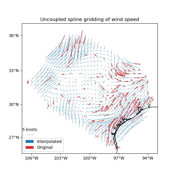
Gridding 2D vectors

We can use verde.Vector to simultaneously process and grid all components of vector data. Each component is processed and gridded separately (see Erizo for an elastically coupled alternative) but we have the convenience of dealing with a single estimator. verde.Vector can be combined with verde.Trend, verde.Spline, and verde.Chain to create a full processing pipeline.

  station_id  longitude  ...  wind_speed_east_knots  wind_speed_north_knots
0        0F2   -97.7756  ...               1.032920               -2.357185
1        11R   -96.3742  ...               1.692155                2.982564
2        2F5  -101.9018  ...              -1.110056               -0.311412
3        3T5   -96.9500  ...               1.695097                3.018448
4        5C1   -98.6946  ...               1.271400                1.090743

[5 rows x 6 columns]
Chain(steps=[('mean',
              BlockReduce(reduction=<function mean at 0x7fd60247e530>,
                          spacing=37000.0)),
             ('trend', Vector(components=[Trend(degree=1), Trend(degree=1)])),
             ('spline',
              Vector(components=[Spline(damping=1e-10, mindist=0),
                                 Spline(damping=1e-10, mindist=0)]))])
/usr/share/miniconda/envs/test/lib/python3.12/site-packages/verde/blockreduce.py:179: FutureWarning: The provided callable <function mean at 0x7fd602476c00> is currently using DataFrameGroupBy.mean. In a future version of pandas, the provided callable will be used directly. To keep current behavior pass the string "mean" instead.
  blocked = pd.DataFrame(columns).groupby("block").aggregate(reduction)
/usr/share/miniconda/envs/test/lib/python3.12/site-packages/verde/blockreduce.py:236: FutureWarning: The provided callable <function mean at 0x7fd602476c00> is currently using DataFrameGroupBy.mean. In a future version of pandas, the provided callable will be used directly. To keep current behavior pass the string "mean" instead.
  grouped = table.groupby("block").aggregate(self.reduction)
/home/runner/work/verde/verde/doc/gallery_src/vector_uncoupled.py:68: FutureWarning: The default scoring will change from R² to negative root mean squared error (RMSE) in Verde 2.0.0. This may change model selection results slightly.
  score = chain.score(*test)
Cross-validation R^2 score: 0.77

import cartopy.crs as ccrs
import matplotlib.pyplot as plt
import numpy as np
import pyproj

import verde as vd

# Fetch the wind speed data from Texas.
data = vd.datasets.fetch_texas_wind()
print(data.head())

# Separate out some of the data into utility variables
coordinates = (data.longitude.values, data.latitude.values)
region = vd.get_region(coordinates)
# Use a Mercator projection because Spline is a Cartesian gridder
projection = pyproj.Proj(proj="merc", lat_ts=data.latitude.mean())

# Split the data into a training and testing set. We'll fit the gridder on the
# training set and use the testing set to evaluate how well the gridder is
# performing.
train, test = vd.train_test_split(
    projection(*coordinates),
    (data.wind_speed_east_knots, data.wind_speed_north_knots),
    random_state=2,
)

# We'll make a 20 arc-minute grid
spacing = 20 / 60

# Chain together a blocked mean to avoid aliasing, a polynomial trend (Spline
# usually requires de-trended data), and finally a Spline for each component.
# Notice that BlockReduce can work on multicomponent data without the use of
# Vector.
chain = vd.Chain(
    [
        ("mean", vd.BlockReduce(np.mean, spacing * 111e3)),
        ("trend", vd.Vector([vd.Trend(degree=1) for i in range(2)])),
        (
            "spline",
            vd.Vector([vd.Spline(damping=1e-10) for i in range(2)]),
        ),
    ]
)
print(chain)

# Fit on the training data
chain.fit(*train)
# And score on the testing data. The best possible score is 1, meaning a
# perfect prediction of the test data.
score = chain.score(*test)
print("Cross-validation R^2 score: {:.2f}".format(score))

# Interpolate the wind speed onto a regular geographic grid and mask the data
# that are outside of the convex hull of the data points.
grid_full = chain.grid(
    region=region,
    spacing=spacing,
    projection=projection,
    dims=["latitude", "longitude"],
)
grid = vd.convexhull_mask(coordinates, grid=grid_full, projection=projection)

# Make maps of the original and gridded wind speed
plt.figure(figsize=(6, 6))
ax = plt.axes(projection=ccrs.Mercator())
ax.set_title("Uncoupled spline gridding of wind speed")
tmp = ax.quiver(
    grid.longitude.values,
    grid.latitude.values,
    grid.east_component.values,
    grid.north_component.values,
    width=0.0015,
    scale=100,
    color="tab:blue",
    transform=ccrs.PlateCarree(),
    label="Interpolated",
)
ax.quiver(
    *coordinates,
    data.wind_speed_east_knots.values,
    data.wind_speed_north_knots.values,
    width=0.003,
    scale=100,
    color="tab:red",
    transform=ccrs.PlateCarree(),
    label="Original",
)
ax.quiverkey(tmp, 0.17, 0.23, 5, label="5 knots", coordinates="figure")
ax.legend(loc="lower left")
# Use an utility function to add tick labels and land and ocean features to the
# map.
vd.datasets.setup_texas_wind_map(ax)
plt.show()