Magnetic airborne survey of the Osborne Mine, Australia

This is a section of a survey acquired in 1990 by the Queensland Government, Australia. The line data have approximately 80 m terrain clearance and 200 m line spacing. The section contains the total field magnetic anomalies associated with the Osborne Mine, Lightning Creek sill complex, and the Brumby prospect.

Original source: Geophysical Acquisition & Processing Section 2019. MIM Data from Mt Isa Inlier, QLD (P1029), magnetic line data, AWAGS levelled. Geoscience Australia, Canberra

Pre-processing: Source code for preparation of the original dataset for redistribution in Ensaio

import pandas as pd
import pygmt

import ensaio

Download and cache the data and return the path to it on disk

fname = ensaio.fetch_osborne_magnetic(version=1)
print(fname)

/home/runner/work/_temp/cache/ensaio/v1/osborne-magnetic.csv.xz

Load the CSV formatted data with pandas

data = pd.read_csv(fname)
data

	flight_line	longitude	latitude	height_orthometric_m	total_field_anomaly_nt
0	5576	140.66411	-21.86833	367	-124
1	5576	140.66403	-21.86832	367	-124
2	5576	140.66394	-21.86832	367	-124
3	5576	140.66385	-21.86832	366	-124
4	5576	140.66377	-21.86832	366	-124
...	...	...	...	...	...
990982	10166	140.50757	-21.87023	382	-67
990983	10166	140.50757	-21.87029	382	-66
990984	10166	140.50758	-21.87034	383	-66
990985	10166	140.50758	-21.87040	383	-66
990986	10166	140.50758	-21.87046	382	-65

990987 rows × 5 columns

Make a PyGMT map with the data points colored by the total field magnetic anomaly.

fig = pygmt.Figure()
fig.basemap(
    projection="M15c",
    region=[
        data.longitude.min(),
        data.longitude.max(),
        data.latitude.min(),
        data.latitude.max(),
    ],
    frame="af",
)
scale = 1500
pygmt.makecpt(cmap="polar+h", series=[-scale, scale], background=True)
fig.plot(
    x=data.longitude,
    y=data.latitude,
    fill=data.total_field_anomaly_nt,
    style="c0.075c",
    cmap=True,
)
fig.colorbar(
    frame='af+l"total field magnetic anomaly [nT]"',
    position="JBC+h+o0/1c+e",
)
fig.show()

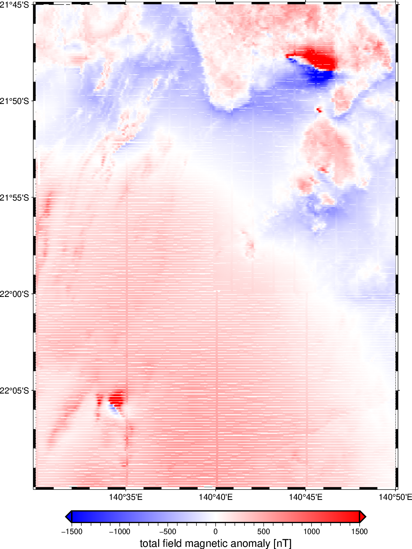
The anomaly at the bottom left is the Osborne Mine. The ones on the top right are the Lightning Creek sill complex (the largest) and the Brumby prospect (one of the smaller anomalies).