A taste of Verde#
Verde offers a wealth of functionality for processing spatial and geophysical data, like bathymetry, GPS, temperature, gravity, or anything else that is measured along a surface. While our main focus is on gridding (interpolating on a regular grid), you’ll also find other things like trend removal, data decimation, spatial cross-validation, and blocked operations.
This example will show you some of what Verde can do to process some data and generate a grid.
The library#
Most classes and functions are available through the verde top level
package. So we can import only that and we’ll have everything Verde has to offer:
import verde as vd
Note
Throughout the documentation we’ll use vd as the alias for
verde.
We’ll also import other modules for this example:
# Standard Scipy stack
import numpy as np
import pandas as pd
import matplotlib.pyplot as plt
# For projecting data
import pyproj
# For plotting data on a map
import pygmt
# For fetching sample datasets
import ensaio
Loading some sample data#
For this example, we’ll download some sample GPS/GNSS velocity data from across
the Alps using ensaio:
path_to_data_file = ensaio.fetch_alps_gps(version=1)
print(path_to_data_file)
/home/runner/.cache/ensaio/v1/alps-gps-velocity.csv.xz
Since our data are in CSV
format, the best way to load them is with pandas:
data = pd.read_csv(path_to_data_file)
data
| station_id | longitude | latitude | height_m | velocity_east_mmyr | velocity_north_mmyr | velocity_up_mmyr | longitude_error_m | latitude_error_m | height_error_m | velocity_east_error_mmyr | velocity_north_error_mmyr | velocity_up_error_mmyr | |
|---|---|---|---|---|---|---|---|---|---|---|---|---|---|
| 0 | ACOM | 13.514900 | 46.547935 | 1774.682 | 0.2 | 1.2 | 1.1 | 0.0005 | 0.0009 | 0.001 | 0.1 | 0.1 | 0.1 |
| 1 | AFAL | 12.174517 | 46.527144 | 2284.085 | -0.7 | 0.9 | 1.3 | 0.0009 | 0.0009 | 0.001 | 0.1 | 0.2 | 0.2 |
| 2 | AGDE | 3.466427 | 43.296383 | 65.785 | -0.2 | -0.2 | 0.1 | 0.0009 | 0.0018 | 0.002 | 0.1 | 0.3 | 0.3 |
| 3 | AGNE | 7.139620 | 45.467942 | 2354.600 | 0.0 | -0.2 | 1.5 | 0.0009 | 0.0036 | 0.004 | 0.2 | 0.6 | 0.5 |
| 4 | AIGL | 3.581261 | 44.121398 | 1618.764 | 0.0 | 0.1 | 0.7 | 0.0009 | 0.0009 | 0.002 | 0.1 | 0.5 | 0.5 |
| ... | ... | ... | ... | ... | ... | ... | ... | ... | ... | ... | ... | ... | ... |
| 181 | WLBH | 7.351299 | 48.415171 | 819.069 | 0.0 | -0.2 | -2.8 | 0.0005 | 0.0009 | 0.001 | 0.1 | 0.2 | 0.2 |
| 182 | WTZR | 12.878911 | 49.144199 | 666.025 | 0.1 | 0.2 | -0.1 | 0.0005 | 0.0005 | 0.001 | 0.1 | 0.1 | 0.1 |
| 183 | ZADA | 15.227590 | 44.113177 | 64.307 | 0.2 | 3.1 | -0.3 | 0.0018 | 0.0036 | 0.004 | 0.2 | 0.4 | 0.4 |
| 184 | ZIMM | 7.465278 | 46.877098 | 956.341 | -0.1 | 0.4 | 1.0 | 0.0005 | 0.0009 | 0.001 | 0.1 | 0.1 | 0.1 |
| 185 | ZOUF | 12.973553 | 46.557221 | 1946.508 | 0.1 | 1.0 | 1.3 | 0.0005 | 0.0009 | 0.001 | 0.1 | 0.1 | 0.1 |
186 rows × 13 columns
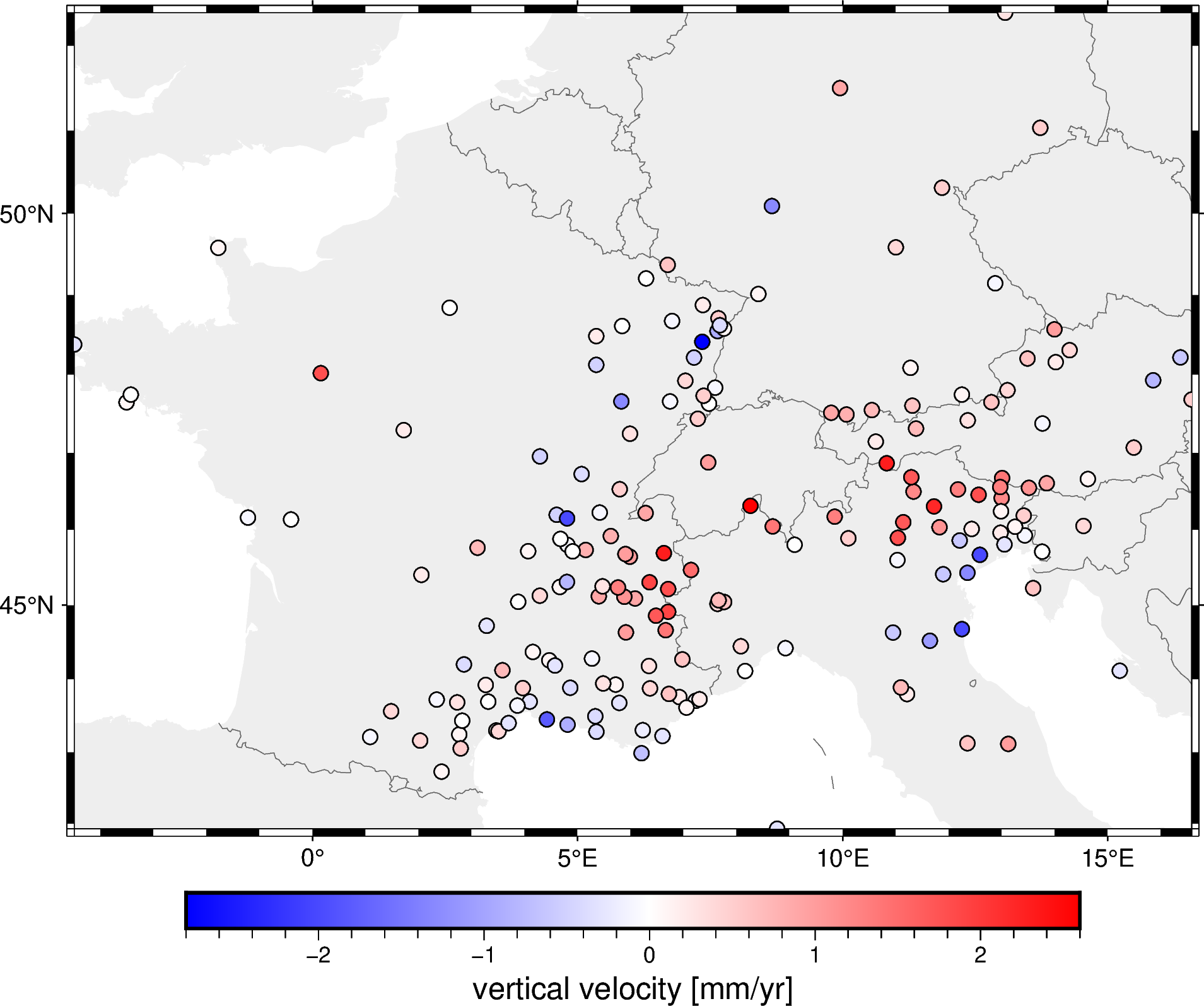
The data are the observed 3D velocity vectors of each GPS/GNSS station in mm/year and show the deformation of the crust that is caused by the subduction in the Alps. For this example, we’ll only the vertical component (but Verde can handle all 3 components as well).
Before we do anything with this data, it would be useful to extract from it the
West, East, South, North bounding box (this is called a region in Verde).
This will help us make a map and can be useful in other operations as well.
Verde offers the function verde.get_region function for doing just
that:
region = vd.get_region([data.longitude, data.latitude])
print(region)
(np.float64(-4.4965935), np.float64(16.5830568), np.float64(41.9274581), np.float64(52.3792981))
Coordinate order
In Verde, coordinates are always given in the order:
West-East, South-North. All functions and classes expect coordinates in
this order. The only exceptions are the dims and shape arguments
that some functions take.
Let’s plot this on a pygmt map so we can see it more clearly:
# Start a figure
fig = pygmt.Figure()
# Add a basemap with the data region, Mercator projection, default frame
# and ticks, color in the continents, and display national borders
fig.coast(
    region=region, projection="M15c", frame="af",
    land="#eeeeee", borders="1/#666666", area_thresh=1e4,
)
# Create a colormap for the velocity
pygmt.makecpt(
    cmap="polar+h",
    series=[data.velocity_up_mmyr.min(), data.velocity_up_mmyr.max()],
)
# Plot colored points for the velocities
fig.plot(
    x=data.longitude,
    y=data.latitude,
    fill=data.velocity_up_mmyr,
    style="c0.2c",
    cmap=True,
    pen="0.5p,black",
)
# Add a colorbar with automatic frame and ticks and a label
fig.colorbar(frame='af+l"vertical velocity [mm/yr]"')
fig.show()
Decimate the data#
You may have noticed that that the spacing between the points is highly variable. This can sometimes cause aliasing problems when gridding and also wastes computation when multiple points would fall on the same grid cell. To avoid all of the this, it’s customary to block average the data first.
Block averaging means splitting the region into blocks (usually with the size
of the desired grid spacing) and then taking the average of all points inside
each block.
In Verde, this is done by verde.BlockMean:
# Desired grid spacing in degrees
spacing = 0.2
blockmean = vd.BlockMean(spacing=spacing)
The verde.BlockMean.filter method applies the blocked average operation
with the given spacing to some data.
It returns for each block: the mean coordinates, the mean data value, and
a weight (we’ll get to that soon).
block_coordinates, block_velocity, block_weights = blockmean.filter(
    coordinates=(data.longitude, data.latitude),
    data=data.velocity_up_mmyr,
)
block_coordinates
(array([ 8.7626159 ,  2.434972  ,  2.7949003 ,  6.2060949 , 12.3557044 ,
        13.1239995 ,  1.0860528 ,  2.02959   ,  2.7660378 ,  3.4876973 ,
         5.3537886 ,  6.2289099 ,  6.6010118 ,  2.8234738 ,  3.6991176 ,
         4.4216344 ,  4.8104624 ,  5.3331971 ,  1.4808917 ,  2.3408725 ,
         2.7275844 ,  3.3143753 ,  3.8648417 ,  4.0958931 ,  5.7869818 ,
         7.0541003 ,  7.26361955,  3.2682596 ,  3.9669648 ,  4.8617726 ,
         5.7173553 ,  6.366692  ,  6.7236848 ,  6.9205745 , 11.0991283 ,
        11.2138006 ,  3.5812609 ,  5.4836986 ,  8.1594175 , 15.2275901 ,
         2.8551187 ,  4.4669187 ,  4.5738468 ,  5.2725628 ,  6.3455153 ,
         6.9770648 ,  4.156319  ,  8.0811275 ,  8.9211444 , 11.6468163 ,
         3.2836469 ,  5.9105951 ,  6.6618686 , 10.9491953 , 12.2494364 ,
         6.4789542 ,  6.7100358 ,  3.8788733 ,  4.2874656 ,  5.3984569 ,
         5.881079  ,  6.0834629 ,  7.6503444 ,  7.7653026 ,  4.665694  ,
         4.7979068 ,  5.4725132 ,  5.7617809 ,  6.358558  ,  6.7100867 ,
        13.5950464 ,  2.0519965 ,  7.1396203 , 11.8960633 , 12.3540792 ,
         4.0678111 ,  4.9058086 ,  5.1521292 ,  5.9021552 ,  5.985685  ,
         6.6282299 , 11.0342814 , 12.5884184 , 13.7635214 ,  3.1110763 ,
         4.6765767 ,  4.8089593 ,  5.624649  ,  9.0956236 , 10.1088147 ,
        11.042103  , 12.2085197 , 13.0525523 , 13.4356375 , -0.4076986 ,
         4.8029182 ,  8.6802049 , 11.1434418 , 11.8270897 , 12.4350216 ,
        12.9790963 , 13.2530207 , 14.543717  , -1.2193156 ,  4.6061776 ,
         5.416495  ,  6.2830311 ,  8.2610005 ,  9.8502544 , 11.7237974 ,
        12.987684  , 13.4160616 ,  5.7956604 , 11.3367981 , 12.174517  ,
        12.5653448 , 13.0011467 , 13.5149004 ,  5.0751405 , 11.2946668 ,
        12.9914523 , 13.850455  , 14.6260666 ,  7.4652781 , 10.8315721 ,
         4.2889755 , 10.6268236 , 15.4934817 ,  1.7196751 ,  5.9893868 ,
        11.3860936 ,  7.2681933 ,  9.7846655 , 10.0725985 , 10.5510003 ,
        12.3594601 , 13.7713212 , -3.5079805 , -3.427339  ,  5.8265567 ,
         6.7456111 ,  7.4288212 , 11.3149642 , 12.2492719 , 12.8075351 ,
        16.5830568 ,  7.0315242 ,  7.5961676 , 13.1104313 , 15.8589121 ,
         0.1552863 ,  5.3508882 , 11.2798716 , 14.0207379 ,  7.1967089 ,
        13.486385  , 14.2830623 , 16.3730836 , -4.4965935 ,  5.3535964 ,
         7.3512992 ,  7.6399038 ,  5.8411017 ,  6.7838184 ,  7.6710324 ,
         7.7624948 , 13.9953591 ,  2.5873124 ,  7.3642111 ,  8.4112604 ,
        12.8789111 ,  6.2915779 ,  6.6996722 , -1.7779594 , 11.0045746 ,
         8.6649682 , 11.8758926 , 13.7296944 ,  9.9505607 , 13.0660927 ]),
 array([41.9274581 , 42.7275495 , 43.0481629 , 42.9832846 , 43.1193923 ,
        43.1119865 , 43.2068502 , 43.1571519 , 43.2419319 , 43.2913725 ,
        43.2787706 , 43.3010132 , 43.2194846 , 43.4313718 , 43.3976493 ,
        43.4491472 , 43.3759731 , 43.4912152 , 43.5606955 , 43.7203399 ,
        43.6809908 , 43.6933643 , 43.6374387 , 43.6923772 , 43.6757239 ,
        43.6114285 , 43.71438235, 43.9198043 , 43.8769014 , 43.8813695 ,
        43.9241573 , 43.873539  , 43.7974659 , 43.7547386 , 43.8855632 ,
        43.7956496 , 44.1213985 , 43.9409571 , 44.1095454 , 44.1131766 ,
        44.1996596 , 44.2554513 , 44.1853354 , 44.2778955 , 44.1772974 ,
        44.2678215 , 44.3692026 , 44.4459918 , 44.4193884 , 44.5199581 ,
        44.7217941 , 44.6328399 , 44.6622451 , 44.6293541 , 44.6769027 ,
        44.8576702 , 44.9103636 , 45.0436188 , 45.124571  , 45.1166293 ,
        45.1107151 , 45.0866148 , 45.0392507 , 45.0415489 , 45.2413805 ,
        45.3071052 , 45.2493163 , 45.2352196 , 45.3041378 , 45.2137781 ,
        45.2260172 , 45.4033539 , 45.4679419 , 45.4111544 , 45.4305709 ,
        45.7156927 , 45.7137762 , 45.7333733 , 45.6776851 , 45.6430025 ,
        45.6914899 , 45.599783  , 45.6684352 , 45.7097578 , 45.7609636 ,
        45.8790852 , 45.7990205 , 45.916077  , 45.802164  , 45.8860062 ,
        45.8935061 , 45.8570112 , 45.805723  , 45.9244697 , 46.1334636 ,
        46.1482756 , 46.0423417 , 46.0981198 , 46.0321389 , 46.0082949 ,
        45.958532  , 46.0374798 , 46.0481344 , 46.158943  , 46.1948277 ,
        46.2247145 , 46.2176766 , 46.3135602 , 46.1700344 , 46.3039483 ,
        46.2407539 , 46.1839611 , 46.528575  , 46.4990246 , 46.527144  ,
        46.4570897 , 46.4141535 , 46.5479352 , 46.7255889 , 46.685116  ,
        46.615732  , 46.6070306 , 46.6614109 , 46.8770983 , 46.8665916 ,
        46.9538414 , 47.14623   , 47.0671307 , 47.2941957 , 47.246882  ,
        47.3129057 , 47.4383509 , 47.5153293 , 47.4925837 , 47.5487161 ,
        47.4182421 , 47.3772563 , 47.6480085 , 47.7461152 , 47.6595708 ,
        47.6596952 , 47.6831756 , 47.6067929 , 47.7474651 , 47.6511983 ,
        47.6836476 , 47.923005  , 47.8339487 , 47.8034215 , 47.9279647 ,
        48.0186173 , 48.1244335 , 48.0861707 , 48.1583438 , 48.2168508 ,
        48.2034179 , 48.309783  , 48.2188572 , 48.3804944 , 48.486154  ,
        48.4151715 , 48.5493608 , 48.6123195 , 48.6751878 , 48.66522695,
        48.5798433 , 48.5698369 , 48.8410585 , 48.8730278 , 49.0112461 ,
        49.1441992 , 49.2039455 , 49.3715652 , 49.5806623 , 49.5864936 ,
        50.0905788 , 50.3129033 , 51.029827  , 51.5002153 , 52.3792981 ]))
In this case, we have uncertainty data for each observation and so we can
pass that as input weights to the block averaging (and compute a
weighted average instead).
The weights should usually be 1 over the uncertainty squared and we need to
let verde.BlockMean know that our input weights are uncertainties.
It’s always recommended to use weights if you have them!
blockmean = vd.BlockMean(spacing=spacing, uncertainty=True)
block_coordinates, block_velocity, block_weights = blockmean.filter(
    coordinates=(data.longitude, data.latitude),
    data=data.velocity_up_mmyr,
    weights=1 / data.velocity_up_error_mmyr**2,
)
What if I don’t have uncertainties?
Don’t worry! Input weights are optional in Verde and can always be ommited.
Block weights
The weights that are returned by verde.BlockMean.filter can be
different things. See verde.BlockMean for a detailed explanation.
In our case, they are 1 over the propagated uncertainty of the mean values
for each block.
These can be used in the gridding process to give less weight to the data
that have higher uncertainties.
Now let’s plot the block-averaged data:
fig = pygmt.Figure()
fig.coast(
    region=region, projection="M15c", frame="af",
    land="#eeeeee", borders="1/#666666", area_thresh=1e4,
)
pygmt.makecpt(
    cmap="polar+h", series=[block_velocity.min(), block_velocity.max()],
)
fig.plot(
    x=block_coordinates[0],
    y=block_coordinates[1],
    fill=block_velocity,
    style="c0.2c",
    cmap=True,
    pen="0.5p,black",
)
fig.colorbar(frame='af+l"vertical velocity [mm/yr]"')
fig.show()

It may not seem like much happened, but if you look closely you’ll see that data points that were closer than the spacing were combined into one.
Project the data#
In this example, we’ll use Verde’s Cartesian interpolators.
So we need to project the geographic data we have to Cartesian coordinates
first.
We’ll use pyproj to create a projection function and convert our
longitude and latitude to easting and northing Mercator projection coordinates.
# Create a Mercator projection with latitude of true scale as the data mean
projection = pyproj.Proj(proj="merc", lat_ts=data.latitude.mean())

easting, northing = projection(block_coordinates[0], block_coordinates[1])
Spline interpolation#
Since our data are relatively small (< 10k points), we can use the
verde.Spline class for bi-harmonic spline interpolation
[Sandwell1987] to get a smooth surface that best fits the data:
# Generate a spline with the default arguments
spline = vd.Spline()
# Fit the spline to our decimated and projected data
spline.fit(
    coordinates=(easting, northing),
    data=block_velocity,
    weights=block_weights,
)
Spline(mindist=0)In a Jupyter environment, please rerun this cell to show the HTML representation or trust the notebook.
On GitHub, the HTML representation is unable to render, please try loading this page with nbviewer.org.
Parameters
| mindist | 0 | |
| damping | None | |
| force_coords | None | |
| engine | 'auto' |
Have more than 10k data?
You may want to use some of our other interpolators instead, like
KNeighbors or Cubic. The bi-harmonic spline
is very memory intensive so avoid using it for >10k data unless you have a
lot of RAM.
Now that we have a fitted spline, we can use it to make predictions at any
location we want using verde.Spline.predict.
For example, we can predict on the original data points to calculate the
residuals and evaluate how well the spline fits our data.
To do this, we’ll have to project the original coordinates first:
prediction = spline.predict(projection(data.longitude, data.latitude))
residuals = data.velocity_up_mmyr - prediction

fig = pygmt.Figure()
fig.coast(
    region=region, projection="M15c", frame="af",
    land="#eeeeee", borders="1/#666666", area_thresh=1e4,
)
pygmt.makecpt(
    cmap="polar+h", series=[residuals.min(), residuals.max()],
)
fig.plot(
    x=data.longitude,
    y=data.latitude,
    fill=residuals,
    style="c0.2c",
    cmap=True,
    pen="0.5p,black",
)
fig.colorbar(frame='af+l"fit residuals [mm/yr]"')
fig.show()
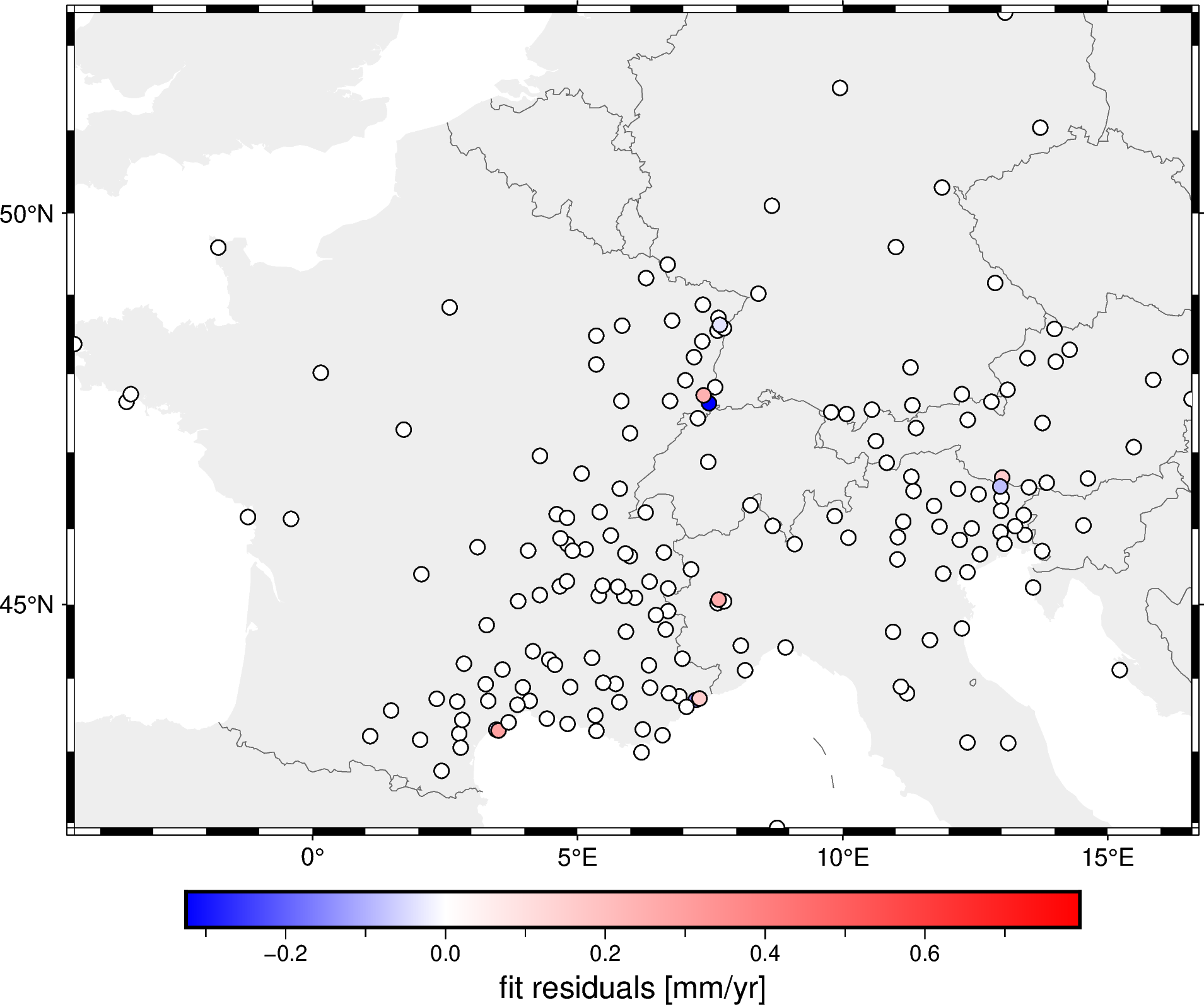
As you can see by the colorbar, the residuals are quite small meaning that the spline fits the decimated data very well.
Generating a grid#
To make a grid using our spline interpolation, we can use
verde.Spline.grid:
# Set the spacing between grid nodes in km
grid = spline.grid(spacing=20e3)
grid
<xarray.Dataset> Size: 42kB
Dimensions:   (northing: 61, easting: 83)
Coordinates:
  * northing  (northing) float64 488B 3.565e+06 3.585e+06 ... 4.758e+06
  * easting   (easting) float64 664B -3.485e+05 -3.285e+05 ... 1.285e+06
Data variables:
    scalars   (northing, easting) float64 41kB -1.83 -1.795 ... -0.08501 -0.1041
Attributes:
metadata: Generated by Spline(mindist=0)The generated grid is an xarray.Dataset and is Cartesian by
default.
The grid contains some metadata and default names for the coordinates and data
variables.
Plotting the grid with matplotlib is as easy as:
# scalars is the default name Verde gives to data variables
grid.scalars.plot()
<matplotlib.collections.QuadMesh at 0x7f13039713d0>
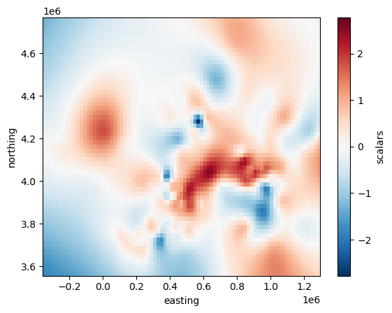
But it’s not that easy to draw borders and coastlines on top of this Cartesian grid.
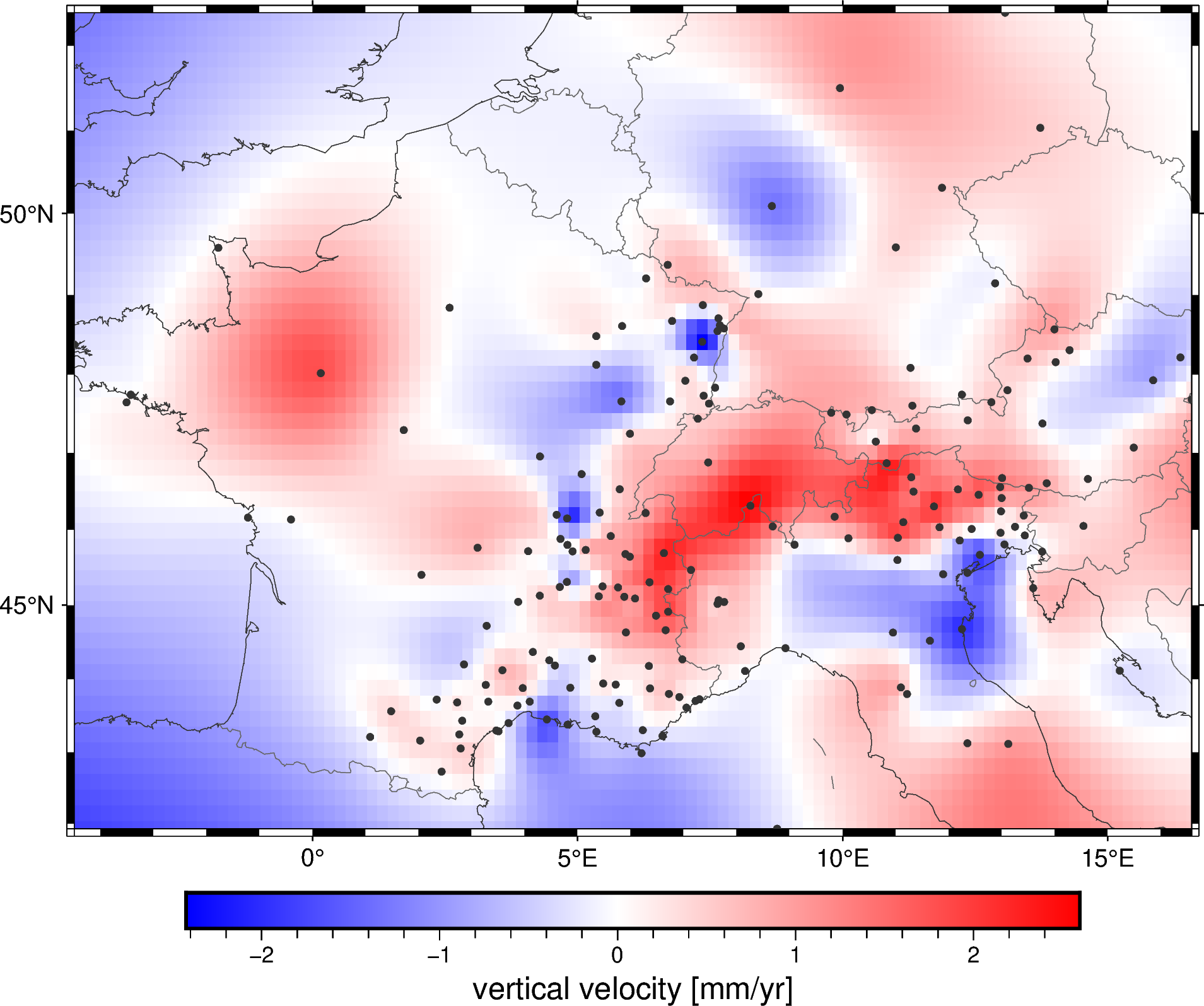
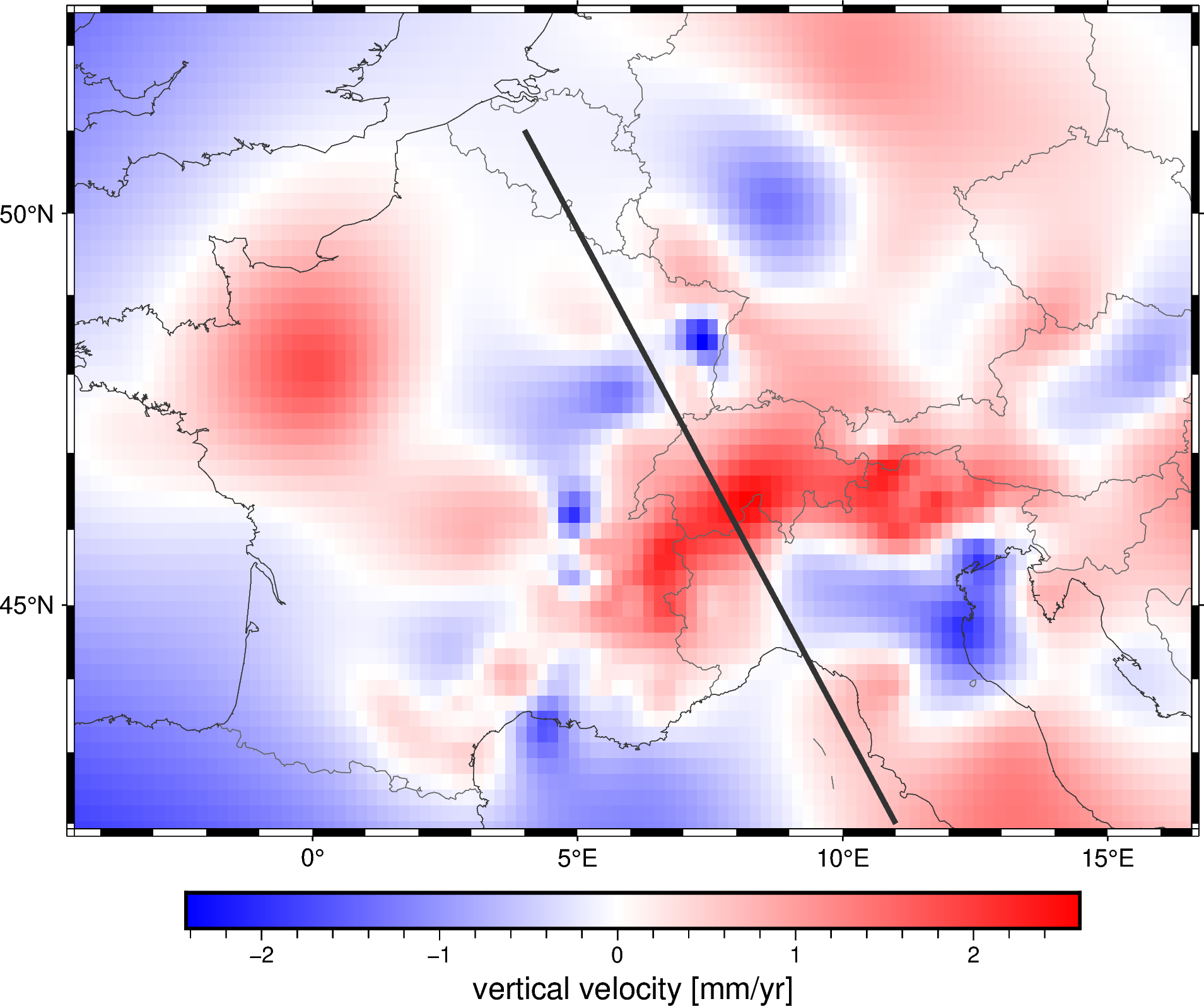
To generate a geographic grid with longitude and latitude, we can pass in the geographic region and the projection used like so:
# Spacing in degrees and customize the names of the dimensions and variables
grid = spline.grid(
    region=region,
    spacing=spacing,
    dims=("latitude", "longitude"),
    data_names="velocity_up",
    projection=projection,  # Our projection function from earlier
)
grid
<xarray.Dataset> Size: 46kB
Dimensions:      (latitude: 53, longitude: 106)
Coordinates:
  * latitude     (latitude) float64 424B 41.93 42.13 42.33 ... 51.98 52.18 52.38
  * longitude    (longitude) float64 848B -4.497 -4.296 -4.095 ... 16.38 16.58
Data variables:
    velocity_up  (latitude, longitude) float64 45kB -1.83 -1.802 ... -0.1041
Attributes:
metadata: Generated by Spline(mindist=0)Plotting a geographic grid is easier done with PyGMT so we can add coastlines and country borders:
fig = pygmt.Figure()
fig.grdimage(grid.velocity_up, cmap="polar+h", projection="M15c")
fig.coast(
    frame="af", shorelines="#333333", borders="1/#666666", area_thresh=1e4,
)
fig.colorbar(frame='af+l"vertical velocity [mm/yr]"')
fig.plot(
    x=data.longitude,
    y=data.latitude,
    fill="#333333",
    style="c0.1c",
)
fig.show()
Did you notice?
The verde.Spline was fitted only once on the input that and we then
used it to generate 3 separate interpolations. In general, fitting is the
most time-consuming part for bi-harmonic splines.
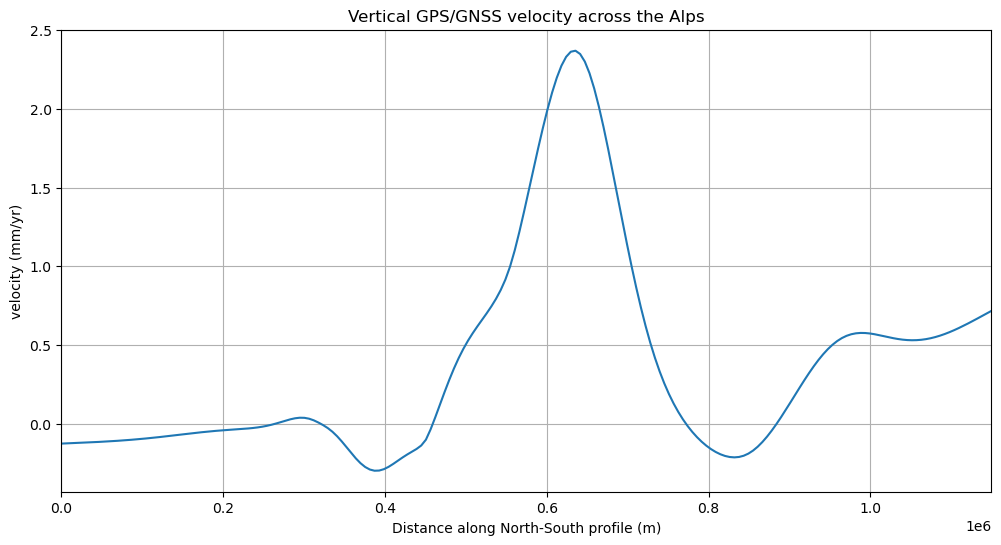
Extracting a profile#
Once we have a fitted spline, we can also use it to predict data along a
profile with the verde.Spline.profile method. For example, let’s
extract a profile that cuts across the Alps:
profile = spline.profile(
    point1=(4, 51),  # longitude, latitude of a point
    point2=(11, 42),
    size=200,  # number of points
    dims=("latitude", "longitude"),
    data_names="velocity_up_mmyr",
    projection=projection,
)
profile
| latitude | longitude | distance | velocity_up_mmyr | |
|---|---|---|---|---|
| 0 | 51.000000 | 4.000000 | 0.000000e+00 | -0.126214 |
| 1 | 50.958517 | 4.035176 | 5.776034e+03 | -0.124948 |
| 2 | 50.916997 | 4.070352 | 1.155207e+04 | -0.123690 |
| 3 | 50.875440 | 4.105528 | 1.732810e+04 | -0.122425 |
| 4 | 50.833845 | 4.140704 | 2.310414e+04 | -0.121140 |
| ... | ... | ... | ... | ... |
| 195 | 42.195756 | 10.859296 | 1.126327e+06 | 0.652267 |
| 196 | 42.146874 | 10.894472 | 1.132103e+06 | 0.668127 |
| 197 | 42.097954 | 10.929648 | 1.137879e+06 | 0.684209 |
| 198 | 42.048996 | 10.964824 | 1.143655e+06 | 0.700388 |
| 199 | 42.000000 | 11.000000 | 1.149431e+06 | 0.716551 |
200 rows × 4 columns
Note
We passed in a projection because our spline is Cartesian but we want to generate a profile between 2 points specified with geographic coordinates. The resulting points will be evenly spaced in the projected coordinates.
The result is a pandas.DataFrame with the coordinates, distance along
the profile, and interpolated data values.
Let’s plot the location of the profile on our map:
fig = pygmt.Figure()
fig.grdimage(grid.velocity_up, cmap="polar+h", projection="M15c")
fig.coast(
    frame="af", shorelines="#333333", borders="1/#666666", area_thresh=1e4,
)
fig.colorbar(frame='af+l"vertical velocity [mm/yr]"')
fig.plot(
    x=profile.longitude,
    y=profile.latitude,
    pen="2p,#333333",
)
fig.show()
Finally, we can plot the profile data using matplotlib:
plt.figure(figsize=(12, 6))
plt.plot(profile.distance, profile.velocity_up_mmyr, "-")
plt.title("Vertical GPS/GNSS velocity across the Alps")
plt.xlabel("Distance along North-South profile (m)")
plt.ylabel("velocity (mm/yr)")
plt.xlim(profile.distance.min(), profile.distance.max())
plt.grid()
plt.show()
Wrapping up#
This covers the basics of using Verde. Most use cases will involve some variation of the following workflow:
Load data (coordinates and data values)
Create a gridder
Fit the gridder to the data
Now go explore the rest of the documentation and try out Verde on your own data!
Questions or comments?
Reach out to us through one of our communication channels! We love hearing from users and are always looking for more people to get involved with developing Verde.