Gridding with splines and weights

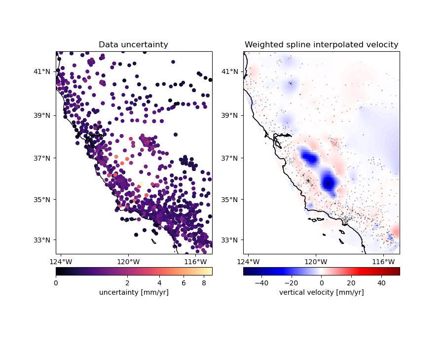
An advantage of using the Green’s functions based verde.Spline over verde.ScipyGridder is that you can assign weights to the data to incorporate the data uncertainties or variance into the gridding. In this example, we’ll see how to combine verde.BlockMean to decimate the data and use weights based on the data uncertainty during gridding.

Chain(steps=[('mean', BlockMean(spacing=9250.0, uncertainty=True)),
             ('spline', Spline(damping=1e-10, mindist=0))])
/home/runner/work/verde/verde/doc/gallery_src/spline_weights.py:58: FutureWarning: The default scoring will change from R² to negative root mean squared error (RMSE) in Verde 2.0.0. This may change model selection results slightly.
  score = chain.score(*test)

Score: 0.819

import cartopy.crs as ccrs
import matplotlib.pyplot as plt
import pyproj
from matplotlib.colors import PowerNorm

import verde as vd

# We'll test this on the California vertical GPS velocity data because it comes
# with the uncertainties
data = vd.datasets.fetch_california_gps()
coordinates = (data.longitude.values, data.latitude.values)

# Use a Mercator projection for our Cartesian gridder
projection = pyproj.Proj(proj="merc", lat_ts=data.latitude.mean())

# Now we can chain a block weighted mean and weighted spline together. We'll
# use uncertainty propagation to calculate the new weights from block mean
# because our data vary smoothly but have different uncertainties.
spacing = 5 / 60  # 5 arc-minutes
chain = vd.Chain(
    [
        ("mean", vd.BlockMean(spacing=spacing * 111e3, uncertainty=True)),
        ("spline", vd.Spline(damping=1e-10)),
    ]
)
print(chain)

# Split the data into a training and testing set. We'll use the training set to
# grid the data and the testing set to validate our spline model. Weights need
# to 1/uncertainty**2 for the error propagation in BlockMean to work.
train, test = vd.train_test_split(
    projection(*coordinates),
    data.velocity_up,
    weights=1 / data.std_up**2,
    random_state=0,
)
# Fit the model on the training set
chain.fit(*train)
# And calculate an R^2 score coefficient on the testing set. The best possible
# score (perfect prediction) is 1. This can tell us how good our spline is at
# predicting data that was not in the input dataset.
score = chain.score(*test)
print("\nScore: {:.3f}".format(score))

# Create a grid of the vertical velocity and mask it to only show points close
# to the actual data.
region = vd.get_region(coordinates)
grid_full = chain.grid(
    region=region,
    spacing=spacing,
    projection=projection,
    dims=["latitude", "longitude"],
    data_names=["velocity"],
)
grid = vd.convexhull_mask(
    (data.longitude, data.latitude), grid=grid_full, projection=projection
)

fig, axes = plt.subplots(
    1, 2, figsize=(9, 7), subplot_kw=dict(projection=ccrs.Mercator())
)
crs = ccrs.PlateCarree()
# Plot the data uncertainties
ax = axes[0]
ax.set_title("Data uncertainty")
# Plot the uncertainties in mm/yr and using a power law for the color scale to
# highlight the smaller values
pc = ax.scatter(
    *coordinates,
    c=data.std_up * 1000,
    s=20,
    cmap="magma",
    transform=crs,
    norm=PowerNorm(gamma=1 / 2)
)
cb = plt.colorbar(pc, ax=ax, orientation="horizontal", pad=0.05)
cb.set_label("uncertainty [mm/yr]")
vd.datasets.setup_california_gps_map(ax, region=region)
# Plot the gridded velocities
ax = axes[1]
ax.set_title("Weighted spline interpolated velocity")
maxabs = vd.maxabs(data.velocity_up) * 1000
pc = (grid.velocity * 1000).plot.pcolormesh(
    ax=ax,
    cmap="seismic",
    vmin=-maxabs,
    vmax=maxabs,
    transform=crs,
    add_colorbar=False,
    add_labels=False,
)
cb = plt.colorbar(pc, ax=ax, orientation="horizontal", pad=0.05)
cb.set_label("vertical velocity [mm/yr]")
ax.scatter(*coordinates, c="black", s=0.5, alpha=0.1, transform=crs)
vd.datasets.setup_california_gps_map(ax, region=region)
ax.coastlines()
plt.show()