verde.Trend

verde.Trend#

class verde.Trend(degree)[source]#

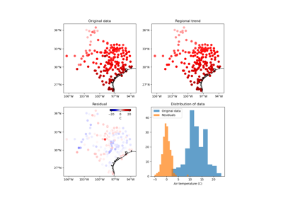
Fit a 2D polynomial trend to spatial data.

The polynomial of degree $N$ is defined as:

\[f(e, n) = \sum\limits_{l=0}^{N}\sum\limits_{m=0}^{N - l} e^l n^m\]

in which $e$ and $n$ are the easting and northing coordinates, respectively.

The trend is estimated through weighted least-squares regression. The Jacobian (design, sensitivity, feature, etc) matrix for the regression is normalized using sklearn.preprocessing.StandardScaler without centering the mean so that the transformation can be undone in the estimated coefficients.

Parameters:

degreeint: The degree of the polynomial. Must be >= 0 (a degree of zero would estimate the mean of the data).

Examples

>>> from verde import grid_coordinates
>>> import numpy as np
>>> coordinates = grid_coordinates((1, 5, -5, -1), shape=(5, 5))
>>> data = 10 + 2*coordinates[0] - 0.4*coordinates[1]
>>> trend = Trend(degree=1).fit(coordinates, data)
>>> print(
...     "Coefficients:",
...     ', '.join(['{:.1f}'.format(i) for i in trend.coef_])
... )
Coefficients: 10.0, 2.0, -0.4
>>> np.allclose(trend.predict(coordinates), data)
True

A zero degree polynomial estimates the mean of the data:

>>> mean = Trend(degree=0).fit(coordinates, data)
>>> np.allclose(mean.predict(coordinates), data.mean())
True
>>> print("Data mean:", '{:.2f}'.format(data.mean()))
Data mean: 17.20
>>> print("Coefficient:", '{:.2f}'.format(mean.coef_[0]))
Coefficient: 17.20

We can use weights to account for outliers or data points with variable uncertainties (see verde.variance_to_weights):

>>> data_out = data.copy()
>>> data_out[2, 2] += 500
>>> weights = np.ones_like(data)
>>> weights[2, 2] = 1e-10
>>> trend_out = Trend(degree=1).fit(coordinates, data_out, weights)
>>> # Still recover the coefficients even with the added outlier
>>> print(
...     "Coefficients:",
...     ', '.join(['{:.1f}'.format(i) for i in trend_out.coef_])
... )
Coefficients: 10.0, 2.0, -0.4
>>> # The residual at the outlier location should be values we added to
>>> # that point
>>> residual = data_out - trend_out.predict(coordinates)
>>> print('{:.2f}'.format(residual[2, 2]))
500.00

Attributes:

coef_array: The estimated polynomial coefficients that fit the observed data.
region_tuple: The boundaries ([W, E, S, N]) of the data used to fit the interpolator. Used as the default region for the grid and scatter methods.

Methods

`filter`(coordinates, data[, weights])	Filter the data through the gridder and produce residuals.
`fit`(coordinates, data[, weights])	Fit the trend to the given data.
`get_metadata_routing`()	Get metadata routing of this object.
`get_params`([deep])	Get parameters for this estimator.
`grid`([region, shape, spacing, dims, ...])	Interpolate the data onto a regular grid.
`jacobian`(coordinates[, dtype])	Make the Jacobian matrix for a 2D polynomial.
`predict`(coordinates)	Evaluate the polynomial trend on the given set of points.
`profile`(point1, point2, size[, dims, ...])	Interpolate data along a profile between two points.
`scatter`([region, size, random_state, dims, ...])	Interpolate values onto a random scatter of points.
`score`(coordinates, data[, weights])	Score the gridder predictions against the given data.
`set_fit_request`(*[, coordinates, data, weights])	Request metadata passed to the `fit` method.
`set_params`(**params)	Set the parameters of this estimator.
`set_predict_request`(*[, coordinates])	Request metadata passed to the `predict` method.
`set_score_request`(*[, coordinates, data, ...])	Request metadata passed to the `score` method.

Attributes#

Trend.data_names_defaults = [('scalars',), ('east_component', 'north_component'), ('east_component', 'north_component', 'vertical_component')]#

Trend.dims = ('northing', 'easting')#

Trend.extra_coords_name = 'extra_coord'#

Methods#

Trend.filter(coordinates, data, weights=None)#

Filter the data through the gridder and produce residuals.

Calls fit on the data, evaluates the residuals (data - predicted data), and returns the coordinates, residuals, and weights.

Not very useful by itself but this interface makes gridders compatible with other processing operations and is used by verde.Chain to join them together (for example, so you can fit a spline on the residuals of a trend).

Parameters:

coordinatestuple of arrays: Arrays with the coordinates of each data point. Should be in the following order: (easting, northing, vertical, …). For the specific definition of coordinate systems and what these names mean, see the class docstring.
dataarray or tuple of arrays: The data values of each data point. If the data has more than one component, data must be a tuple of arrays (one for each component).
weightsNone or array or tuple of arrays: If not None, then the weights assigned to each data point. If more than one data component is provided, you must provide a weights array for each data component (if not None).

Returns:

coordinates, residuals, weights: The coordinates and weights are same as the input. Residuals are the input data minus the predicted data.

Trend.fit(coordinates, data, weights=None)[source]#

Fit the trend to the given data.

The data region is captured and used as default for the grid and scatter methods.

All input arrays must have the same shape.

Parameters:

coordinatestuple of arrays: Arrays with the coordinates of each data point. Should be in the following order: (easting, northing, vertical, …). Only easting and northing will be used, all subsequent coordinates will be ignored.
dataarray: The data values of each data point.
weightsNone or array: If not None, then the weights assigned to each data point. Typically, this should be 1 over the data uncertainty squared.

Returns:

self: Returns this estimator instance for chaining operations.

Trend.get_metadata_routing()#

Get metadata routing of this object.

Please check User Guide on how the routing mechanism works.

Returns:

routingMetadataRequest: A MetadataRequest encapsulating routing information.

Trend.get_params(deep=True)#

Get parameters for this estimator.

Parameters:

deepbool, default=True: If True, will return the parameters for this estimator and contained subobjects that are estimators.

Returns:

paramsdict: Parameter names mapped to their values.

Trend.grid(region=None, shape=None, spacing=None, dims=None, data_names=None, projection=None, coordinates=None, **kwargs)#

Interpolate the data onto a regular grid.

The grid can be specified by two methods:

Pass the actual coordinates of the grid points, as generated by verde.grid_coordinates or from an existing xarray.Dataset grid.
Let the method define a new grid by either passing the number of points in each dimension (the shape) or by the grid node spacing. If the interpolator collected the input data region, then it will be used if region=None. Otherwise, you must specify the grid region. See verde.grid_coordinates for details. Other arguments for verde.grid_coordinates can be passed as extra keyword arguments (kwargs) to this method.

Use the dims and data_names arguments to set custom names for the dimensions and the data field(s) in the output xarray.Dataset. Default names will be provided if none are given.

Parameters:

regionlist = [W, E, S, N]: The west, east, south, and north boundaries of a given region. Use only if coordinates is None.
shapetuple = (n_north, n_east) or None: The number of points in the South-North and West-East directions, respectively. Use only if coordinates is None.
spacingtuple = (s_north, s_east) or None: The grid spacing in the South-North and West-East directions, respectively. Use only if coordinates is None.
dimslist or None: The names of the northing and easting data dimensions, respectively, in the output grid. Default is determined from the dims attribute of the class. Must be defined in the following order: northing dimension, easting dimension. NOTE: This is an exception to the “easting” then “northing” pattern but is required for compatibility with xarray.
data_namesstr, list or None: The name(s) of the data variables in the output grid. Defaults to 'scalars' for scalar data, ['east_component', 'north_component'] for 2D vector data, and ['east_component', 'north_component', 'vertical_component'] for 3D vector data.
projectioncallable or None: If not None, then should be a callable object projection(easting, northing) -> (proj_easting, proj_northing) that takes in easting and northing coordinate arrays and returns projected northing and easting coordinate arrays. This function will be used to project the generated grid coordinates before passing them into predict. For example, you can use this to generate a geographic grid from a Cartesian gridder.
coordinatestuple of arrays: Tuple of arrays containing the coordinates of the grid in the following order: (easting, northing, vertical, …). The easting and northing arrays could be 1d or 2d arrays, if they are 2d they must be part of a meshgrid. If coordinates are passed, region, shape, and spacing are ignored.

Returns:

gridxarray.Dataset: The interpolated grid. Metadata about the interpolator is written to the attrs attribute.

See also

verde.grid_coordinates: Generate the coordinate values for the grid.

Trend.jacobian(coordinates, dtype='float64')[source]#

Make the Jacobian matrix for a 2D polynomial.

Each column of the Jacobian is easting**i * northing**j for each (i, j) pair in the polynomial.

Parameters:

coordinatestuple of arrays: Arrays with the coordinates of each data point. Should be in the following order: (easting, northing, vertical, …). Only easting and northing will be used, all subsequent coordinates will be ignored.
dtypestr or numpy dtype: The type of the output Jacobian numpy array.

Returns:

jacobian2D array: The (n_data, n_coefficients) Jacobian matrix.

Examples

>>> import numpy as np
>>> east = np.linspace(0, 4, 5)
>>> north = np.linspace(-5, -1, 5)
>>> print(Trend(degree=1).jacobian((east, north), dtype=int))
[[ 1  0 -5]
 [ 1  1 -4]
 [ 1  2 -3]
 [ 1  3 -2]
 [ 1  4 -1]]
>>> print(Trend(degree=2).jacobian((east, north), dtype=int))
[[ 1  0 -5  0  0 25]
 [ 1  1 -4  1 -4 16]
 [ 1  2 -3  4 -6  9]
 [ 1  3 -2  9 -6  4]
 [ 1  4 -1 16 -4  1]]

Trend.predict(coordinates)[source]#

Evaluate the polynomial trend on the given set of points.

Requires a fitted estimator (see fit).

Parameters:

coordinatestuple of arrays: Arrays with the coordinates of each data point. Should be in the following order: (easting, northing, vertical, …). Only easting and northing will be used, all subsequent coordinates will be ignored.

Returns:

dataarray: The trend values evaluated on the given points.

Trend.profile(point1, point2, size, dims=None, data_names=None, projection=None, **kwargs)#

Interpolate data along a profile between two points.

Generates the profile along a straight line assuming Cartesian distances. Point coordinates are generated by verde.profile_coordinates. Other arguments for this function can be passed as extra keyword arguments (kwargs) to this method.

Use the dims and data_names arguments to set custom names for the dimensions and the data field(s) in the output pandas.DataFrame. Default names are provided.

Includes the calculated Cartesian distance from point1 for each data point in the profile.

To specify point1 and point2 in a coordinate system that would require projection to Cartesian (geographic longitude and latitude, for example), use the projection argument. With this option, the input points will be projected using the given projection function prior to computations. The generated Cartesian profile coordinates will be projected back to the original coordinate system. Note that the profile points are evenly spaced in projected coordinates, not the original system (e.g., geographic).

Warning

The profile calculation method with a projection has changed in Verde 1.4.0. Previous versions generated coordinates (assuming they were Cartesian) and projected them afterwards. This led to “distances” being incorrectly handled and returned in unprojected coordinates. For example, if projection is from geographic to Mercator, the distances would be “angles” (incorrectly calculated as if they were Cartesian). After 1.4.0, point1 and point2 are projected prior to generating coordinates for the profile, guaranteeing that distances are properly handled in a Cartesian system. With this change, the profile points are now evenly spaced in projected coordinates and the distances are returned in projected coordinates as well.

Parameters:

point1tuple: The easting and northing coordinates, respectively, of the first point.
point2tuple: The easting and northing coordinates, respectively, of the second point.
sizeint: The number of points to generate.
dimslist or None: The names of the northing and easting data dimensions, respectively, in the output dataframe. Default is determined from the dims attribute of the class. Must be defined in the following order: northing dimension, easting dimension. NOTE: This is an exception to the “easting” then “northing” pattern but is required for compatibility with xarray.
data_namesstr, list or None: The name(s) of the data variables in the output dataframe. Defaults to 'scalars' for scalar data, ['east_component', 'north_component'] for 2D vector data, and ['east_component', 'north_component', 'vertical_component'] for 3D vector data.
projectioncallable or None: If not None, then should be a callable object projection(easting, northing, inverse=False) -> (proj_easting, proj_northing) that takes in easting and northing coordinate arrays and returns projected northing and easting coordinate arrays. Should also take an optional keyword argument inverse (default to False) that if True will calculate the inverse transform instead. This function will be used to project the profile end points before generating coordinates and passing them into predict. It will also be used to undo the projection of the coordinates before returning the results.

Returns:

tablepandas.DataFrame: The interpolated values along the profile.

Trend.scatter(region=None, size=300, random_state=0, dims=None, data_names=None, projection=None, **kwargs)#

Interpolate values onto a random scatter of points.

Point coordinates are generated by verde.scatter_points. Other arguments for this function can be passed as extra keyword arguments (kwargs) to this method.

If the interpolator collected the input data region, then it will be used if region=None. Otherwise, you must specify the grid region.

Use the dims and data_names arguments to set custom names for the dimensions and the data field(s) in the output pandas.DataFrame. Default names are provided.

Warning

The scatter method is deprecated and will be removed in Verde 2.0.0. Use verde.scatter_points and the predict method instead.

Parameters:

regionlist = [W, E, S, N]: The west, east, south, and north boundaries of a given region.
sizeint: The number of points to generate.
random_statenumpy.random.RandomState or an int seed: A random number generator used to define the state of the random permutations. Use a fixed seed to make sure computations are reproducible. Use None to choose a seed automatically (resulting in different numbers with each run).
dimslist or None: The names of the northing and easting data dimensions, respectively, in the output dataframe. Default is determined from the dims attribute of the class. Must be defined in the following order: northing dimension, easting dimension. NOTE: This is an exception to the “easting” then “northing” pattern but is required for compatibility with xarray.
data_namesstr, list or None: The name(s) of the data variables in the output dataframe. Defaults to 'scalars' for scalar data, ['east_component', 'north_component'] for 2D vector data, and ['east_component', 'north_component', 'vertical_component'] for 3D vector data.
projectioncallable or None: If not None, then should be a callable object projection(easting, northing) -> (proj_easting, proj_northing) that takes in easting and northing coordinate arrays and returns projected northing and easting coordinate arrays. This function will be used to project the generated scatter coordinates before passing them into predict. For example, you can use this to generate a geographic scatter from a Cartesian gridder.

Returns:

tablepandas.DataFrame: The interpolated values on a random set of points.

Trend.score(coordinates, data, weights=None)#

Score the gridder predictions against the given data.

Calculates the R^2 coefficient of determination of between the predicted values and the given data values. A maximum score of 1 means a perfect fit. The score can be negative.

Warning

The default scoring will change from R² to negative root mean squared error (RMSE) in Verde 2.0.0. This may change model selection results slightly. The negative version will be used to maintain the behaviour of larger scores being better, which is more compatible with current model selection code.

If the data has more than 1 component, the scores of each component will be averaged.

Parameters:

coordinatestuple of arrays: Arrays with the coordinates of each data point. Should be in the following order: (easting, northing, vertical, …). For the specific definition of coordinate systems and what these names mean, see the class docstring.
dataarray or tuple of arrays: The data values of each data point. If the data has more than one component, data must be a tuple of arrays (one for each component).
weightsNone or array or tuple of arrays: If not None, then the weights assigned to each data point. If more than one data component is provided, you must provide a weights array for each data component (if not None).

Returns:

scorefloat: The R^2 score

Request metadata passed to the fit method.

Note that this method is only relevant if enable_metadata_routing=True (see sklearn.set_config). Please see User Guide on how the routing mechanism works.

The options for each parameter are:

True: metadata is requested, and passed to fit if provided. The request is ignored if metadata is not provided.
False: metadata is not requested and the meta-estimator will not pass it to fit.
None: metadata is not requested, and the meta-estimator will raise an error if the user provides it.
str: metadata should be passed to the meta-estimator with this given alias instead of the original name.

The default (sklearn.utils.metadata_routing.UNCHANGED) retains the existing request. This allows you to change the request for some parameters and not others.

New in version 1.3.

Note

This method is only relevant if this estimator is used as a sub-estimator of a meta-estimator, e.g. used inside a Pipeline. Otherwise it has no effect.

Parameters:

coordinatesstr, True, False, or None, default=sklearn.utils.metadata_routing.UNCHANGED: Metadata routing for coordinates parameter in fit.
datastr, True, False, or None, default=sklearn.utils.metadata_routing.UNCHANGED: Metadata routing for data parameter in fit.
weightsstr, True, False, or None, default=sklearn.utils.metadata_routing.UNCHANGED: Metadata routing for weights parameter in fit.

Returns:

selfobject: The updated object.

Trend.set_params(**params)#

Set the parameters of this estimator.

The method works on simple estimators as well as on nested objects (such as Pipeline). The latter have parameters of the form <component>__<parameter> so that it’s possible to update each component of a nested object.

Parameters:

**paramsdict: Estimator parameters.

Returns:

selfestimator instance: Estimator instance.

Trend.set_predict_request(*, coordinates: bool | None | str = '$UNCHANGED$') → Trend#

Request metadata passed to the predict method.

Note that this method is only relevant if enable_metadata_routing=True (see sklearn.set_config). Please see User Guide on how the routing mechanism works.

The options for each parameter are:

True: metadata is requested, and passed to predict if provided. The request is ignored if metadata is not provided.
False: metadata is not requested and the meta-estimator will not pass it to predict.
None: metadata is not requested, and the meta-estimator will raise an error if the user provides it.
str: metadata should be passed to the meta-estimator with this given alias instead of the original name.

The default (sklearn.utils.metadata_routing.UNCHANGED) retains the existing request. This allows you to change the request for some parameters and not others.

New in version 1.3.

Note

This method is only relevant if this estimator is used as a sub-estimator of a meta-estimator, e.g. used inside a Pipeline. Otherwise it has no effect.

Parameters:

coordinatesstr, True, False, or None, default=sklearn.utils.metadata_routing.UNCHANGED: Metadata routing for coordinates parameter in predict.

Returns:

selfobject: The updated object.

Request metadata passed to the score method.

Note that this method is only relevant if enable_metadata_routing=True (see sklearn.set_config). Please see User Guide on how the routing mechanism works.

The options for each parameter are:

True: metadata is requested, and passed to score if provided. The request is ignored if metadata is not provided.
False: metadata is not requested and the meta-estimator will not pass it to score.
None: metadata is not requested, and the meta-estimator will raise an error if the user provides it.
str: metadata should be passed to the meta-estimator with this given alias instead of the original name.

The default (sklearn.utils.metadata_routing.UNCHANGED) retains the existing request. This allows you to change the request for some parameters and not others.

New in version 1.3.

Note

This method is only relevant if this estimator is used as a sub-estimator of a meta-estimator, e.g. used inside a Pipeline. Otherwise it has no effect.

Parameters:

coordinatesstr, True, False, or None, default=sklearn.utils.metadata_routing.UNCHANGED: Metadata routing for coordinates parameter in score.
datastr, True, False, or None, default=sklearn.utils.metadata_routing.UNCHANGED: Metadata routing for data parameter in score.
weightsstr, True, False, or None, default=sklearn.utils.metadata_routing.UNCHANGED: Metadata routing for weights parameter in score.

Returns: