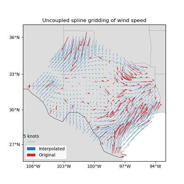
Gridding 2D vectors

We can use verde.Vector to simultaneously process and grid all components of vector data. Each component is processed and gridded separately (see Erizo for an elastically coupled alternative) but we have the convenience of dealing with a single estimator. verde.Vector can be combined with verde.Trend, verde.Spline, and verde.Chain to create a full processing pipeline.

Out:

  station_id  longitude  ...  wind_speed_east_knots  wind_speed_north_knots
0        0F2   -97.7756  ...               1.032920               -2.357185
1        11R   -96.3742  ...               1.692155                2.982564
2        2F5  -101.9018  ...              -1.110056               -0.311412
3        3T5   -96.9500  ...               1.695097                3.018448
4        5C1   -98.6946  ...               1.271400                1.090743

[5 rows x 6 columns]
Chain(steps=[('mean',
              BlockReduce(reduction=<function mean at 0x7fdf232ca1e0>,
                          spacing=37000.0)),
             ('trend', Vector(components=[Trend(degree=1), Trend(degree=1)])),
             ('spline',
              Vector(components=[Spline(damping=1e-10, mindist=500000.0),
                                 Spline(damping=1e-10, mindist=500000.0)]))])
Cross-validation R^2 score: 0.78
/home/travis/miniconda/envs/testing/lib/python3.6/site-packages/cartopy/mpl/geoaxes.py:1752: RuntimeWarning: invalid value encountered in less
  u, v = self.projection.transform_vectors(t, x, y, u, v)
/home/travis/miniconda/envs/testing/lib/python3.6/site-packages/cartopy/mpl/geoaxes.py:1752: RuntimeWarning: invalid value encountered in greater
  u, v = self.projection.transform_vectors(t, x, y, u, v)
/home/travis/miniconda/envs/testing/lib/python3.6/site-packages/cartopy/mpl/geoaxes.py:782: MatplotlibDeprecationWarning: Passing the minor parameter of set_xticks() positionally is deprecated since Matplotlib 3.2; the parameter will become keyword-only two minor releases later.
  return super(GeoAxes, self).set_xticks(xticks, minor)
/home/travis/miniconda/envs/testing/lib/python3.6/site-packages/cartopy/mpl/geoaxes.py:829: MatplotlibDeprecationWarning: Passing the minor parameter of set_yticks() positionally is deprecated since Matplotlib 3.2; the parameter will become keyword-only two minor releases later.
  return super(GeoAxes, self).set_yticks(yticks, minor)
/home/travis/build/fatiando/verde/examples/vector_uncoupled.py:99: UserWarning: Tight layout not applied. The left and right margins cannot be made large enough to accommodate all axes decorations.
  plt.tight_layout()

import matplotlib.pyplot as plt
import cartopy.crs as ccrs
import numpy as np
import pyproj
import verde as vd


# Fetch the wind speed data from Texas.
data = vd.datasets.fetch_texas_wind()
print(data.head())

# Separate out some of the data into utility variables
coordinates = (data.longitude.values, data.latitude.values)
region = vd.get_region(coordinates)
# Use a Mercator projection because Spline is a Cartesian gridder
projection = pyproj.Proj(proj="merc", lat_ts=data.latitude.mean())

# Split the data into a training and testing set. We'll fit the gridder on the training
# set and use the testing set to evaluate how well the gridder is performing.
train, test = vd.train_test_split(
    projection(*coordinates),
    (data.wind_speed_east_knots, data.wind_speed_north_knots),
    random_state=2,
)

# We'll make a 20 arc-minute grid
spacing = 20 / 60

# Chain together a blocked mean to avoid aliasing, a polynomial trend (Spline usually
# requires de-trended data), and finally a Spline for each component. Notice that
# BlockReduce can work on multicomponent data without the use of Vector.
chain = vd.Chain(
    [
        ("mean", vd.BlockReduce(np.mean, spacing * 111e3)),
        ("trend", vd.Vector([vd.Trend(degree=1) for i in range(2)])),
        (
            "spline",
            vd.Vector([vd.Spline(damping=1e-10, mindist=500e3) for i in range(2)]),
        ),
    ]
)
print(chain)

# Fit on the training data
chain.fit(*train)
# And score on the testing data. The best possible score is 1, meaning a perfect
# prediction of the test data.
score = chain.score(*test)
print("Cross-validation R^2 score: {:.2f}".format(score))

# Interpolate the wind speed onto a regular geographic grid and mask the data that are
# outside of the convex hull of the data points.
grid_full = chain.grid(
    region, spacing=spacing, projection=projection, dims=["latitude", "longitude"]
)
grid = vd.convexhull_mask(coordinates, grid=grid_full, projection=projection)

# Make maps of the original and gridded wind speed
plt.figure(figsize=(6, 6))
ax = plt.axes(projection=ccrs.Mercator())
ax.set_title("Uncoupled spline gridding of wind speed")
tmp = ax.quiver(
    grid.longitude.values,
    grid.latitude.values,
    grid.east_component.values,
    grid.north_component.values,
    width=0.0015,
    scale=100,
    color="tab:blue",
    transform=ccrs.PlateCarree(),
    label="Interpolated",
)
ax.quiver(
    *coordinates,
    data.wind_speed_east_knots.values,
    data.wind_speed_north_knots.values,
    width=0.003,
    scale=100,
    color="tab:red",
    transform=ccrs.PlateCarree(),
    label="Original",
)
ax.quiverkey(tmp, 0.17, 0.23, 5, label="5 knots", coordinates="figure")
ax.legend(loc="lower left")
# Use an utility function to add tick labels and land and ocean features to the map.
vd.datasets.setup_texas_wind_map(ax)
plt.tight_layout()
plt.show()