Projection of gridded data

Sometimes gridded data products need to be projected before they can be used. For example, you might want to project the topography of Antarctica from geographic latitude and longitude to a planar polar stereographic projection before doing your analysis. When projecting, the data points will likely not fall on a regular grid anymore and must be interpolated (re-sampled) onto a new grid.

The verde.project_grid function automates this process using the interpolation methods available in Verde. An input grid (xarray.DataArray) is interpolated onto a new grid in the given pyproj projection. The function takes care of choosing a default grid spacing and region, running a blocked mean to avoid spatial aliasing (using BlockReduce), and masking the points in the new grid that aren’t constrained by the original data (using convexhull_mask).

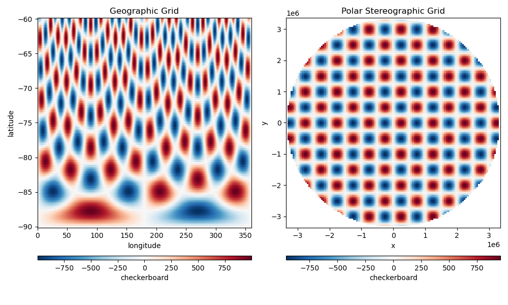
In this example, we’ll generate a synthetic geographic grid with a checkerboard pattern around the South pole. We’ll project the grid to South Polar Stereographic, revealing the checkered pattern of the data.

Note

The interpolation methods are limited to what is available in Verde and there is only support for single 2D grids. For more sophisticated use cases, you might want to try pyresample instead.

Out:

Geographic grid:
<xarray.Dataset>
Dimensions:       (latitude: 121, longitude: 1441)
Coordinates:
  * longitude     (longitude) float64 0.0 0.25 0.5 0.75 ... 359.5 359.8 360.0
  * latitude      (latitude) float64 -90.0 -89.75 -89.5 ... -60.5 -60.25 -60.0
Data variables:
    checkerboard  (latitude, longitude) float64 0.0 0.0 0.0 ... 90.55 45.51 -0.0
Attributes:
    metadata:  Generated by CheckerBoard(region=(-3333134.027630277, 3333134....

Projected grid:
<xarray.DataArray 'checkerboard' (y: 134, x: 134)>
array([[nan, nan, nan, ..., nan, nan, nan],
       [nan, nan, nan, ..., nan, nan, nan],
       [nan, nan, nan, ..., nan, nan, nan],
       ...,
       [nan, nan, nan, ..., nan, nan, nan],
       [nan, nan, nan, ..., nan, nan, nan],
       [nan, nan, nan, ..., nan, nan, nan]])
Coordinates:
  * x        (x) float64 -3.333e+06 -3.283e+06 ... 3.283e+06 3.333e+06
  * y        (y) float64 -3.333e+06 -3.283e+06 ... 3.283e+06 3.333e+06
Attributes:
    metadata:  Generated by Chain(steps=[('mean',\n              BlockReduce(...

import numpy as np
import matplotlib.pyplot as plt
import pyproj
import verde as vd


# We'll use synthetic data near the South pole to highlight the effects of the
# projection. EPSG 3031 is a South Polar Stereographic projection.
projection = pyproj.Proj("epsg:3031")

# Create a synthetic geographic grid using a checkerboard pattern
region = (0, 360, -90, -60)
spacing = 0.25
wavelength = 10 * 1e5  # The size of the cells in the checkerboard
checkerboard = vd.datasets.CheckerBoard(
    region=vd.project_region(region, projection), w_east=wavelength, w_north=wavelength
)
data = checkerboard.grid(
    region=region,
    spacing=spacing,
    projection=projection,
    data_names=["checkerboard"],
    dims=("latitude", "longitude"),
)
print("Geographic grid:")
print(data)

# Do the projection while setting the output grid spacing (in projected meters). Set
# the coordinates names to x and y since they aren't really "northing" or
# "easting".
polar_data = vd.project_grid(
    data.checkerboard, projection, spacing=0.5 * 1e5, dims=("y", "x")
)
print("\nProjected grid:")
print(polar_data)

# Plot the original and projected grids
fig, (ax1, ax2) = plt.subplots(1, 2, figsize=(10, 6))
data.checkerboard.plot(
    ax=ax1, cbar_kwargs=dict(orientation="horizontal", aspect=50, pad=0.1)
)
ax1.set_title("Geographic Grid")
polar_data.plot(ax=ax2, cbar_kwargs=dict(orientation="horizontal", aspect=50, pad=0.1))
ax2.set_title("Polar Stereographic Grid")
plt.tight_layout()
plt.show()