Geographic Coordinates

Most gridders and processing methods in Verde operate under the assumption that the data coordinates are Cartesian. To process data in geographic (longitude and latitude) coordinates, we must first project them. There are different ways of doing this in Python but most of them rely on the PROJ library. We’ll use pyproj to access PROJ directly and handle the projection operations.

import pyproj
import numpy as np
import matplotlib.pyplot as plt
import cartopy.crs as ccrs
import verde as vd

With pyproj, we can create functions that will project our coordinates to and from different coordinate systems. For our Baja California bathymetry data, we’ll use a Mercator projection.

data = vd.datasets.fetch_baja_bathymetry()
# We're choosing the latitude of true scale as the mean latitude of our dataset.
projection = pyproj.Proj(proj="merc", lat_ts=data.latitude.mean())

The Proj object is a callable (meaning that it behaves like a function) that will take longitude and latitude and return easting and northing coordinates.

# pyproj doesn't play well with Pandas so we need to convert to numpy arrays
proj_coords = projection(data.longitude.values, data.latitude.values)
print(proj_coords)

Out:

(array([-11749316.65303046, -11748999.90777981, -11748682.14077029, ...,
       -11749178.71558259, -11749531.22239381, -11749882.70744613]), array([2905766.05183735, 2905457.83817751, 2905148.48639437, ...,
       2579612.89349502, 2580017.48641078, 2580422.09116873]))

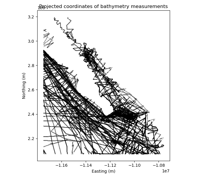
We can plot our projected coordinates using matplotlib.

plt.figure(figsize=(7, 6))
plt.title("Projected coordinates of bathymetry measurements")
# Plot the bathymetry data locations as black dots
plt.plot(proj_coords[0], proj_coords[1], ".k", markersize=0.5)
plt.xlabel("Easting (m)")
plt.ylabel("Northing (m)")
plt.gca().set_aspect("equal")
plt.tight_layout()
plt.show()

Cartesian grids

Now we can use verde.BlockReduce and verde.Spline on our projected coordinates. We’ll specify the desired grid spacing as degrees and convert it to Cartesian using the 1 degree approx. 111 km rule-of-thumb.

spacing = 10 / 60
reducer = vd.BlockReduce(np.median, spacing=spacing * 111e3)
filter_coords, filter_bathy = reducer.filter(proj_coords, data.bathymetry_m)
spline = vd.Spline().fit(filter_coords, filter_bathy)

If we now call verde.Spline.grid we’ll get back a grid evenly spaced in projected Cartesian coordinates.

grid = spline.grid(spacing=spacing * 111e3, data_names=["bathymetry"])
print("Cartesian grid:")
print(grid)

Out:

Cartesian grid:
<xarray.Dataset>
Dimensions:     (easting: 54, northing: 61)
Coordinates:
  * easting     (easting) float64 -1.175e+07 -1.173e+07 ... -1.077e+07
  * northing    (northing) float64 2.074e+06 2.093e+06 ... 3.171e+06 3.19e+06
Data variables:
    bathymetry  (northing, easting) float64 -3.635e+03 -3.727e+03 ... 8.87e+03
Attributes:
    metadata:  Generated by Spline()

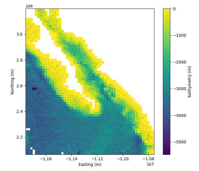
We’ll mask our grid using verde.distance_mask to get rid of all the spurious solutions far away from the data points.

grid = vd.distance_mask(proj_coords, maxdist=30e3, grid=grid)

plt.figure(figsize=(7, 6))
plt.title("Gridded bathymetry in Cartesian coordinates")
pc = grid.bathymetry.plot.pcolormesh(cmap="viridis", vmax=0, add_colorbar=False)
plt.colorbar(pc).set_label("bathymetry (m)")
plt.plot(filter_coords[0], filter_coords[1], ".k", markersize=0.5)
plt.xlabel("Easting (m)")
plt.ylabel("Northing (m)")
plt.gca().set_aspect("equal")
plt.tight_layout()
plt.show()

Geographic grids

The Cartesian grid that we generated won’t be evenly spaced if we convert the coordinates back to geographic latitude and longitude. Verde gridders allow you to generate an evenly spaced grid in geographic coordinates through the projection argument of the grid method.

By providing a projection function (like our pyproj projection object), Verde will generate coordinates for a regular grid and then pass them through the projection function before predicting data values. This way, you can generate a grid in a coordinate system other than the one you used to fit the spline.

# Get the geographic bounding region of the data
region = vd.get_region((data.longitude, data.latitude))
print("Data region in degrees:", region)

# Specify the region and spacing in degrees and a projection function
grid_geo = spline.grid(
    region=region,
    spacing=spacing,
    projection=projection,
    dims=["latitude", "longitude"],
    data_names=["bathymetry"],
)
print("Geographic grid:")
print(grid_geo)

Out:

Data region in degrees: (245.0, 254.705, 20.0, 29.99131)
Geographic grid:
<xarray.Dataset>
Dimensions:     (latitude: 61, longitude: 59)
Coordinates:
  * longitude   (longitude) float64 245.0 245.2 245.3 ... 254.4 254.5 254.7
  * latitude    (latitude) float64 20.0 20.17 20.33 20.5 ... 29.66 29.82 29.99
Data variables:
    bathymetry  (latitude, longitude) float64 -3.621e+03 ... 9.001e+03
Attributes:
    metadata:  Generated by Spline()

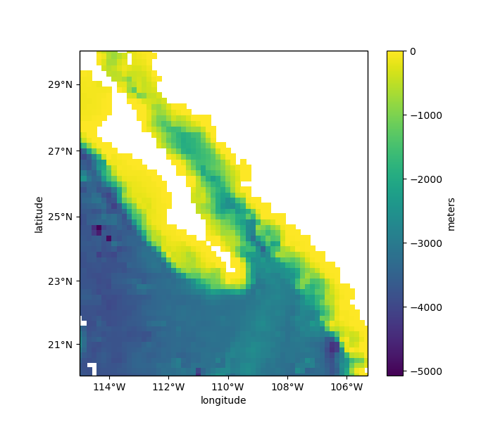
Notice that grid has longitude and latitude coordinates and slightly different number of points than the Cartesian grid.

The verde.distance_mask function also supports the projection argument and will project the coordinates before calculating distances.

grid_geo = vd.distance_mask(
    (data.longitude, data.latitude), maxdist=30e3, grid=grid_geo, projection=projection
)

Now we can use the Cartopy library to plot our geographic grid.

plt.figure(figsize=(7, 6))
ax = plt.axes(projection=ccrs.Mercator())
ax.set_title("Geographic grid of bathymetry")
pc = grid_geo.bathymetry.plot.pcolormesh(
    ax=ax, transform=ccrs.PlateCarree(), vmax=0, zorder=-1, add_colorbar=False
)
plt.colorbar(pc).set_label("meters")
vd.datasets.setup_baja_bathymetry_map(ax, land=None)
plt.show()

Out:

/home/travis/miniconda/envs/testing/lib/python3.6/site-packages/cartopy/mpl/geoaxes.py:782: MatplotlibDeprecationWarning: Passing the minor parameter of set_xticks() positionally is deprecated since Matplotlib 3.2; the parameter will become keyword-only two minor releases later.
  return super(GeoAxes, self).set_xticks(xticks, minor)
/home/travis/miniconda/envs/testing/lib/python3.6/site-packages/cartopy/mpl/geoaxes.py:829: MatplotlibDeprecationWarning: Passing the minor parameter of set_yticks() positionally is deprecated since Matplotlib 3.2; the parameter will become keyword-only two minor releases later.
  return super(GeoAxes, self).set_yticks(yticks, minor)

Profiles

For profiles, things are a bit different. The projection is applied to the input points before coordinates are generated. So the profile will be evenly spaced in projected coordinates, not geographic coordinates. This is to avoid issues with calculating distances on a sphere.

The coordinates returned by the profile method will be in geographic coordinates, so projections given to profile must take an inverse argument so we can undo the projection.

The main utility of using a projection with profile is being able to pass in points in geographic coordinates and get coordinates back in that same system (making it easier to plot on a map).

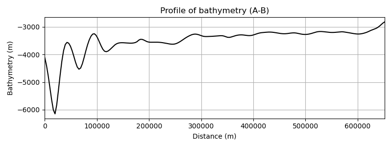
To generate a profile cutting across our bathymetry data, we can use longitude and latitude points taken from the map above).

start = (-114.5, 24.7)
end = (-110, 20.5)
profile = spline.profile(
    point1=start,
    point2=end,
    size=200,
    projection=projection,
    dims=("latitude", "longitude"),
    data_names=["bathymetry"],
)
print(profile)

Out:

      latitude   longitude       distance   bathymetry
0    24.700000 -114.500000       0.000000 -4115.540284
1    24.679226 -114.477387    3276.548360 -4397.069051
2    24.658449 -114.454774    6553.096720 -4766.953632
3    24.637668 -114.432161    9829.645080 -5198.947539
4    24.616884 -114.409548   13106.193440 -5639.303392
..         ...         ...            ...          ...
195  20.585669 -110.090452  638926.930221 -3016.467546
196  20.564257 -110.067839  642203.478581 -2969.351778
197  20.542841 -110.045226  645480.026941 -2914.069304
198  20.521422 -110.022613  648756.575301 -2859.557816
199  20.500000 -110.000000  652033.123661 -2818.101947

[200 rows x 4 columns]

Plot the profile location on our geographic grid from above.

plt.figure(figsize=(7, 6))
ax = plt.axes(projection=ccrs.Mercator())
ax.set_title("Profile location")
pc = grid_geo.bathymetry.plot.pcolormesh(
    ax=ax, transform=ccrs.PlateCarree(), vmax=0, zorder=-1, add_colorbar=False
)
plt.colorbar(pc).set_label("meters")
ax.plot(profile.longitude, profile.latitude, "-k", transform=ccrs.PlateCarree())
ax.text(start[0], start[1], "A", transform=ccrs.PlateCarree())
ax.text(end[0], end[1], "B", transform=ccrs.PlateCarree())
vd.datasets.setup_baja_bathymetry_map(ax, land=None)
plt.show()

Out:

/home/travis/miniconda/envs/testing/lib/python3.6/site-packages/cartopy/mpl/geoaxes.py:782: MatplotlibDeprecationWarning: Passing the minor parameter of set_xticks() positionally is deprecated since Matplotlib 3.2; the parameter will become keyword-only two minor releases later.
  return super(GeoAxes, self).set_xticks(xticks, minor)
/home/travis/miniconda/envs/testing/lib/python3.6/site-packages/cartopy/mpl/geoaxes.py:829: MatplotlibDeprecationWarning: Passing the minor parameter of set_yticks() positionally is deprecated since Matplotlib 3.2; the parameter will become keyword-only two minor releases later.
  return super(GeoAxes, self).set_yticks(yticks, minor)

And finally plot the profile.

plt.figure(figsize=(8, 3))
ax = plt.axes()
ax.set_title("Profile of bathymetry (A-B)")
ax.plot(profile.distance, profile.bathymetry, "-k")
ax.set_xlabel("Distance (m)")
ax.set_ylabel("Bathymetry (m)")
ax.set_xlim(profile.distance.min(), profile.distance.max())
ax.grid()
plt.tight_layout()
plt.show()