Note
Click here to download the full example code
Grid Coordinates
Creating the coordinates for regular grids in Verde is done using the
verde.grid_coordinates function. It creates a set of regularly spaced points in
both the west-east and south-north directions, i.e. a two-dimensional spatial grid. These
points are then used by the Verde gridders to interpolate between data points. As such, all
.grid methods (like verde.Spline.grid) take as input the configuration parameters
for verde.grid_coordinates. The grid can be specified either by the number of points
in each dimension (the shape) or by the grid node spacing.
import numpy as np
import matplotlib.pyplot as plt
import verde as vd
from matplotlib.patches import Rectangle
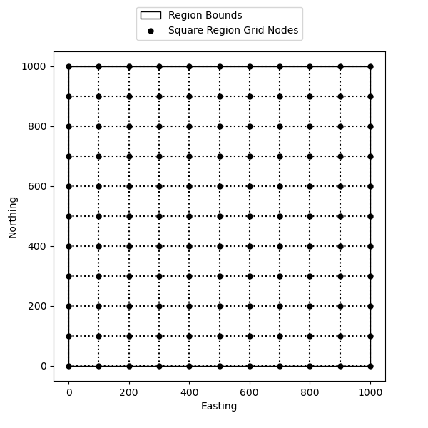
First let’s create a region that is 1000 units west-east and 1000 units south-north, and we will set an initial spacing to 100 units.
We can check the dimensions of the grid coordinates. The region is 1000 units and the spacing is 100 units, so the shape of the segments is 10x10. However, the number of grid nodes in this case is one more than the number of segments. So our grid coordinates have a shape of 11x11.
print(easting.shape, northing.shape)
Out:
(11, 11) (11, 11)
Let’s define two functions to visualize the region bounds and grid points
def plot_region(ax, region):
    "Plot the region as a solid line."
    west, east, south, north = region
    ax.add_patch(
        plt.Rectangle((west, south), east, north, fill=None, label="Region Bounds")
    )


def plot_grid(ax, coordinates, linestyles="dotted", region=None, pad=50, **kwargs):
    "Plot the grid coordinates as dots and lines."
    data_region = vd.get_region(coordinates)
    ax.vlines(
        coordinates[0][0],
        ymin=data_region[2],
        ymax=data_region[3],
        linestyles=linestyles,
        zorder=0,
    )
    ax.hlines(
        coordinates[1][:, 1],
        xmin=data_region[0],
        xmax=data_region[1],
        linestyles=linestyles,
        zorder=0,
    )
    ax.scatter(*coordinates, **kwargs)
    if pad:
        padded = vd.pad_region(region, pad=pad)
        plt.xlim(padded[:2])
        plt.ylim(padded[2:])
Visualize our region and grid coordinates using our functions
plt.figure(figsize=(6, 6))
ax = plt.subplot(111)
plot_region(ax=ax, region=region)
plot_grid(
    ax=ax,
    coordinates=(easting, northing),
    region=region,
    label="Square Region Grid Nodes",
    marker=".",
    color="black",
    s=100,
)

plt.xlabel("Easting")
plt.ylabel("Northing")
plt.legend(loc="upper center", bbox_to_anchor=(0.5, 1.15))
plt.show()
Adjusting region boundaries when creating the grid coordinates
Now let’s change our spacing to 300 units. Because the range of the west-east and south-north boundaries are not multiples of 300, we must choose to change either:
the boundaries of the region in order to fit the spacing, or
the spacing in order to fit the region boundaries.
We could tell verde.grid_coordinates to adjust the region boundaries by
passing adjust="region".
spacing = 300
region_easting, region_northing = vd.grid_coordinates(
    region=region, spacing=spacing, adjust="region"
)
print(region_easting.shape, region_northing.shape)
Out:
(4, 4) (4, 4)
With the spacing set at 300 units and a 4 by 4 grid of regular dimensions,
verde.grid_coordinates calculates the spatial location of each
grid point and adjusts the region so that the maximum northing and maximum
easting values are divisible by the spacing. In this example, both the easting and
northing have 3 segments (4 nodes) that are each 300 units long, meaning the easting
and northing span from 0 to 900. Both dimensions are divisible
by 300.
print(region_easting)
print(region_northing)
Out:
[[  0. 300. 600. 900.]
 [  0. 300. 600. 900.]
 [  0. 300. 600. 900.]
 [  0. 300. 600. 900.]]
[[  0.   0.   0.   0.]
 [300. 300. 300. 300.]
 [600. 600. 600. 600.]
 [900. 900. 900. 900.]]
By default, if adjust is not assigned to "region" or "spacing",
then verde.grid_coordinates will adjust the spacing. With the adjust
parameter set to spacing verde.grid_coordinates creates grid nodes
in a similar manner as when it adjusts the region. However, it doesn’t readjust
the region so that it is divisble by the spacing before creating the grid.
This means the grid will have the same number of grid points no matter if
the adjust parameter is set to region or spacing.
Adjusting spacing when creating the grid
Now let’s adjust the spacing of the grid points by passing adjust="spacing"
to verde.grid_coordinates.
spacing_easting, spacing_northing = vd.grid_coordinates(
    region=region, spacing=spacing, adjust="spacing"
)
print(spacing_easting.shape, spacing_northing.shape)
Out:
(4, 4) (4, 4)
However the regular spacing between the grid points is no longer 300 units.
print(spacing_easting)
print(spacing_northing)
Out:
[[   0.          333.33333333  666.66666667 1000.        ]
 [   0.          333.33333333  666.66666667 1000.        ]
 [   0.          333.33333333  666.66666667 1000.        ]
 [   0.          333.33333333  666.66666667 1000.        ]]
[[   0.            0.            0.            0.        ]
 [ 333.33333333  333.33333333  333.33333333  333.33333333]
 [ 666.66666667  666.66666667  666.66666667  666.66666667]
 [1000.         1000.         1000.         1000.        ]]
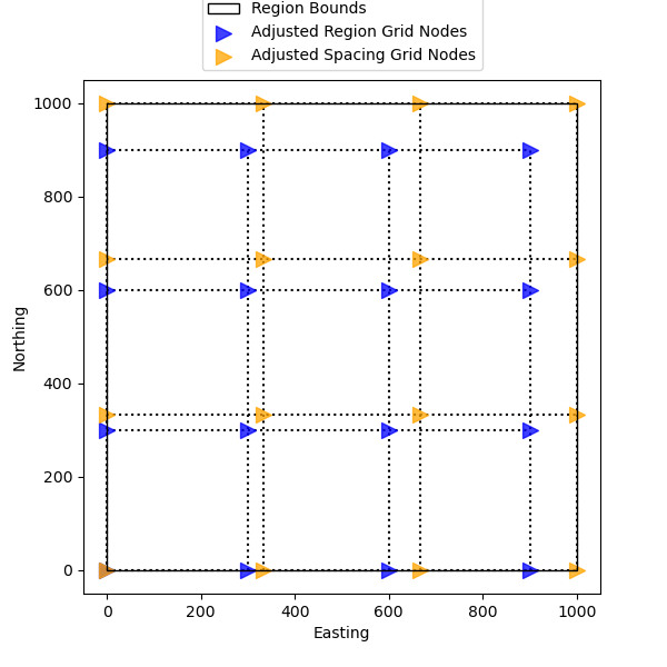
Visualize the different adjustments
Let’s visualize the difference between the original region bounds, the adjusted region grid nodes, and the adjusted spacing grid nodes. Note the adjusted spacing grid nodes keep the original region, while the adjusted region grid nodes on the north and east side of the region have moved.
plt.figure(figsize=(6, 6))
ax = plt.subplot(111)
plot_region(ax=ax, region=region)
plot_grid(
    ax=ax,
    coordinates=(region_easting, region_northing),
    region=region,
    label="Adjusted Region Grid Nodes",
    marker=">",
    color="blue",
    alpha=0.75,
    s=100,
)
plot_grid(
    ax=ax,
    coordinates=(spacing_easting, spacing_northing),
    region=region,
    label="Adjusted Spacing Grid Nodes",
    marker=">",
    color="orange",
    alpha=0.75,
    s=100,
)
plt.xlabel("Easting")
plt.ylabel("Northing")
plt.legend(loc="upper center", bbox_to_anchor=(0.5, 1.18))
plt.show()
Pixel Registration
Pixel registration locates the grid points in the middle of the grid segments rather than in the corner of each grid node.
First, let’s take our 1000x1000 region and use the 100 unit spacing from the first
example and set the pixel_register parameter to True. Without pixel
registration our grid should have dimensions of 11x11. With pixel registration we
expect the dimensions of the grid to be the dimensions of the non-registered grid
minus one, or equal to the number of segments between the grid points in the
non-registered grid (10x10).
spacing = 100
pixel_easting, pixel_northing = vd.grid_coordinates(
    region=region, spacing=spacing, pixel_register=True
)
print(pixel_easting.shape, pixel_northing.shape)
Out:
(10, 10) (10, 10)
And we can check the coordinates for the grid points with pixel registration.
print(pixel_easting)
print(pixel_northing)
Out:
[[ 50. 150. 250. 350. 450. 550. 650. 750. 850. 950.]
 [ 50. 150. 250. 350. 450. 550. 650. 750. 850. 950.]
 [ 50. 150. 250. 350. 450. 550. 650. 750. 850. 950.]
 [ 50. 150. 250. 350. 450. 550. 650. 750. 850. 950.]
 [ 50. 150. 250. 350. 450. 550. 650. 750. 850. 950.]
 [ 50. 150. 250. 350. 450. 550. 650. 750. 850. 950.]
 [ 50. 150. 250. 350. 450. 550. 650. 750. 850. 950.]
 [ 50. 150. 250. 350. 450. 550. 650. 750. 850. 950.]
 [ 50. 150. 250. 350. 450. 550. 650. 750. 850. 950.]
 [ 50. 150. 250. 350. 450. 550. 650. 750. 850. 950.]]
[[ 50.  50.  50.  50.  50.  50.  50.  50.  50.  50.]
 [150. 150. 150. 150. 150. 150. 150. 150. 150. 150.]
 [250. 250. 250. 250. 250. 250. 250. 250. 250. 250.]
 [350. 350. 350. 350. 350. 350. 350. 350. 350. 350.]
 [450. 450. 450. 450. 450. 450. 450. 450. 450. 450.]
 [550. 550. 550. 550. 550. 550. 550. 550. 550. 550.]
 [650. 650. 650. 650. 650. 650. 650. 650. 650. 650.]
 [750. 750. 750. 750. 750. 750. 750. 750. 750. 750.]
 [850. 850. 850. 850. 850. 850. 850. 850. 850. 850.]
 [950. 950. 950. 950. 950. 950. 950. 950. 950. 950.]]
If we set pixel_register to False the function will return the grid
coordinates of the nodes instead of pixel centers, resulting in an extra point in each direction.
easting, northing = vd.grid_coordinates(
    region=region, spacing=spacing, pixel_register=False
)
print(easting.shape, northing.shape)
Out:
(11, 11) (11, 11)
Again we can check the coordinates for grid points with spacing adjustment.
Out:
[[   0.  100.  200.  300.  400.  500.  600.  700.  800.  900. 1000.]
 [   0.  100.  200.  300.  400.  500.  600.  700.  800.  900. 1000.]
 [   0.  100.  200.  300.  400.  500.  600.  700.  800.  900. 1000.]
 [   0.  100.  200.  300.  400.  500.  600.  700.  800.  900. 1000.]
 [   0.  100.  200.  300.  400.  500.  600.  700.  800.  900. 1000.]
 [   0.  100.  200.  300.  400.  500.  600.  700.  800.  900. 1000.]
 [   0.  100.  200.  300.  400.  500.  600.  700.  800.  900. 1000.]
 [   0.  100.  200.  300.  400.  500.  600.  700.  800.  900. 1000.]
 [   0.  100.  200.  300.  400.  500.  600.  700.  800.  900. 1000.]
 [   0.  100.  200.  300.  400.  500.  600.  700.  800.  900. 1000.]
 [   0.  100.  200.  300.  400.  500.  600.  700.  800.  900. 1000.]]
[[   0.    0.    0.    0.    0.    0.    0.    0.    0.    0.    0.]
 [ 100.  100.  100.  100.  100.  100.  100.  100.  100.  100.  100.]
 [ 200.  200.  200.  200.  200.  200.  200.  200.  200.  200.  200.]
 [ 300.  300.  300.  300.  300.  300.  300.  300.  300.  300.  300.]
 [ 400.  400.  400.  400.  400.  400.  400.  400.  400.  400.  400.]
 [ 500.  500.  500.  500.  500.  500.  500.  500.  500.  500.  500.]
 [ 600.  600.  600.  600.  600.  600.  600.  600.  600.  600.  600.]
 [ 700.  700.  700.  700.  700.  700.  700.  700.  700.  700.  700.]
 [ 800.  800.  800.  800.  800.  800.  800.  800.  800.  800.  800.]
 [ 900.  900.  900.  900.  900.  900.  900.  900.  900.  900.  900.]
 [1000. 1000. 1000. 1000. 1000. 1000. 1000. 1000. 1000. 1000. 1000.]]
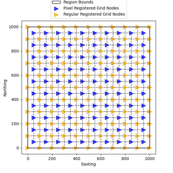
Lastly, we can visualize the pixel-registered grid points to see where they fall within the original region bounds.
plt.figure(figsize=(6, 6))
ax = plt.subplot(111)
plot_region(ax=ax, region=region)
plot_grid(
    ax=ax,
    coordinates=(pixel_easting, pixel_northing),
    region=region,
    label="Pixel Registered Grid Nodes",
    marker=">",
    color="blue",
    alpha=0.75,
    s=100,
)
plot_grid(
    ax=ax,
    coordinates=(easting, northing),
    region=region,
    label="Regular Registered Grid Nodes",
    marker=">",
    color="orange",
    alpha=0.75,
    s=100,
)

plt.xlabel("Easting")
plt.ylabel("Northing")
plt.legend(loc="upper center", bbox_to_anchor=(0.5, 1.18))
plt.show()
Extra Coordinates
In some cases, you might need an additional coordinate such as a height or a time
that is associated with your coordinate grid. The extra_coords parameter
in verde.grid_coordinates creates an extra coordinate array that is the same
shape as the coordinate grid, but contains a constant value. For example, let’s
add a constant height of 1000 units and time of 1 to our coordinate grid.
easting, northing, height, time = vd.grid_coordinates(
    region=region, spacing=spacing, extra_coords=[1000, 1]
)

print(easting.shape, northing.shape, height.shape, time.shape)
Out:
(11, 11) (11, 11) (11, 11) (11, 11)
And we can print the height array to verify that it is correct
print(height)
Out:
[[1000. 1000. 1000. 1000. 1000. 1000. 1000. 1000. 1000. 1000. 1000.]
 [1000. 1000. 1000. 1000. 1000. 1000. 1000. 1000. 1000. 1000. 1000.]
 [1000. 1000. 1000. 1000. 1000. 1000. 1000. 1000. 1000. 1000. 1000.]
 [1000. 1000. 1000. 1000. 1000. 1000. 1000. 1000. 1000. 1000. 1000.]
 [1000. 1000. 1000. 1000. 1000. 1000. 1000. 1000. 1000. 1000. 1000.]
 [1000. 1000. 1000. 1000. 1000. 1000. 1000. 1000. 1000. 1000. 1000.]
 [1000. 1000. 1000. 1000. 1000. 1000. 1000. 1000. 1000. 1000. 1000.]
 [1000. 1000. 1000. 1000. 1000. 1000. 1000. 1000. 1000. 1000. 1000.]
 [1000. 1000. 1000. 1000. 1000. 1000. 1000. 1000. 1000. 1000. 1000.]
 [1000. 1000. 1000. 1000. 1000. 1000. 1000. 1000. 1000. 1000. 1000.]
 [1000. 1000. 1000. 1000. 1000. 1000. 1000. 1000. 1000. 1000. 1000.]]
And we can print the time array as well
print(time)
Out:
[[1. 1. 1. 1. 1. 1. 1. 1. 1. 1. 1.]
 [1. 1. 1. 1. 1. 1. 1. 1. 1. 1. 1.]
 [1. 1. 1. 1. 1. 1. 1. 1. 1. 1. 1.]
 [1. 1. 1. 1. 1. 1. 1. 1. 1. 1. 1.]
 [1. 1. 1. 1. 1. 1. 1. 1. 1. 1. 1.]
 [1. 1. 1. 1. 1. 1. 1. 1. 1. 1. 1.]
 [1. 1. 1. 1. 1. 1. 1. 1. 1. 1. 1.]
 [1. 1. 1. 1. 1. 1. 1. 1. 1. 1. 1.]
 [1. 1. 1. 1. 1. 1. 1. 1. 1. 1. 1.]
 [1. 1. 1. 1. 1. 1. 1. 1. 1. 1. 1.]
 [1. 1. 1. 1. 1. 1. 1. 1. 1. 1. 1.]]
Total running time of the script: ( 0 minutes 0.357 seconds)