5. Rescale coordinates to a different region#

Translating and stretching sets of points can sometimes be useful, for example to produce synthetic data based on real data sampling. This operation is basically rescaling a set of coordinates to a different region (bounding box), and can be done with function bordado.rescale_coordinates.

import ensaio
import pygmt
import pandas as pd
import bordado as bd

We’ll use the Southern Africa gravity dataset as an example, which is downloaded using ensaio.fetch_southern_africa_gravity:

fname = ensaio.fetch_southern_africa_gravity(version=1)
data = pd.read_csv(fname)
data

	longitude	latitude	height_sea_level_m	gravity_mgal
0	18.34444	-34.12971	32.2	979656.12
1	18.36028	-34.08833	592.5	979508.21
2	18.37418	-34.19583	18.4	979666.46
3	18.40388	-34.23972	25.0	979671.03
4	18.41112	-34.16444	228.7	979616.11
...	...	...	...	...
14354	21.22500	-17.95833	1053.1	978182.09
14355	21.27500	-17.98333	1033.3	978183.09
14356	21.70833	-17.99166	1041.8	978182.69
14357	21.85000	-17.95833	1033.3	978193.18
14358	21.98333	-17.94166	1022.6	978211.38

14359 rows × 4 columns

Let’s retrieve the original bounding box (region) of the data:

coordinates = (data.longitude, data.latitude)
region = bd.get_region(coordinates)
print(region)

(11.90833, 32.74667, -34.996, -17.33333)

And now we can plot the data along with coastlines so we can better locate it:

fig = pygmt.Figure()
pygmt.makecpt(
    cmap="viridis",
    series=[data.gravity_mgal.min(), data.gravity_mgal.max()],
)
fig.plot(
    x=coordinates[0],
    y=coordinates[1],
    fill=data.gravity_mgal,
    cmap=True,
    style="c0.04c",
    projection="M15c",
    region=region,
)
fig.coast(
    shorelines=True,
    water="royalblue4",
    area_thresh=1e4,
    frame="af",
)
fig.colorbar(frame=["af+lOriginal data", "y+lmGal"])
fig.show()

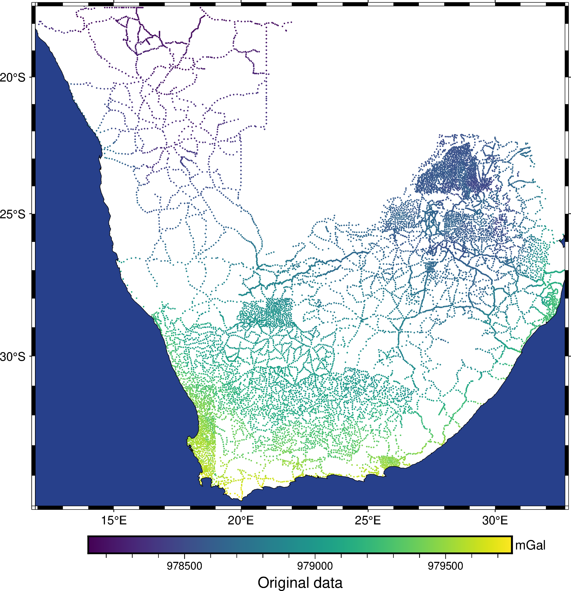
The dataset covers the entire Southern tip of Africa in point. But let’s say we want to translate it to the Amazon region of South America and stretch in latitude a bit. To do so, we define a new region and call rescale_coordinates like so:

new_region = [-70, -50, -30, 10]
rescaled = bd.rescale_coordinates(coordinates, new_region)
print(rescaled)

(array([-63.8228189 , -63.80761615, -63.79427536, ..., -60.59426039,
       -60.45828986, -60.33032382], shape=(14359,)), array([-28.03814486, -27.94443309, -28.18788439, ...,   8.50910423,
         8.58458546,   8.62233739], shape=(14359,)))

The coordinates are now made to be contained in the new_region but retaining relative positioning between them. Let’s plot the rescaled data on a map to visualize:

fig = pygmt.Figure()
pygmt.makecpt(
    cmap="viridis",
    series=[data.gravity_mgal.min(), data.gravity_mgal.max()],
)
fig.plot(
    x=rescaled[0],
    y=rescaled[1],
    fill=data.gravity_mgal,
    cmap=True,
    style="c0.04c",
    projection="M15c",
    region=bd.pad_region(new_region, pad=(10, 5)),
)
fig.coast(
    shorelines=True,
    water="royalblue4",
    area_thresh=1e4,
    frame="afg",
)
fig.colorbar(frame=["af+lRescaled data", "y+lmGal"])
fig.show()

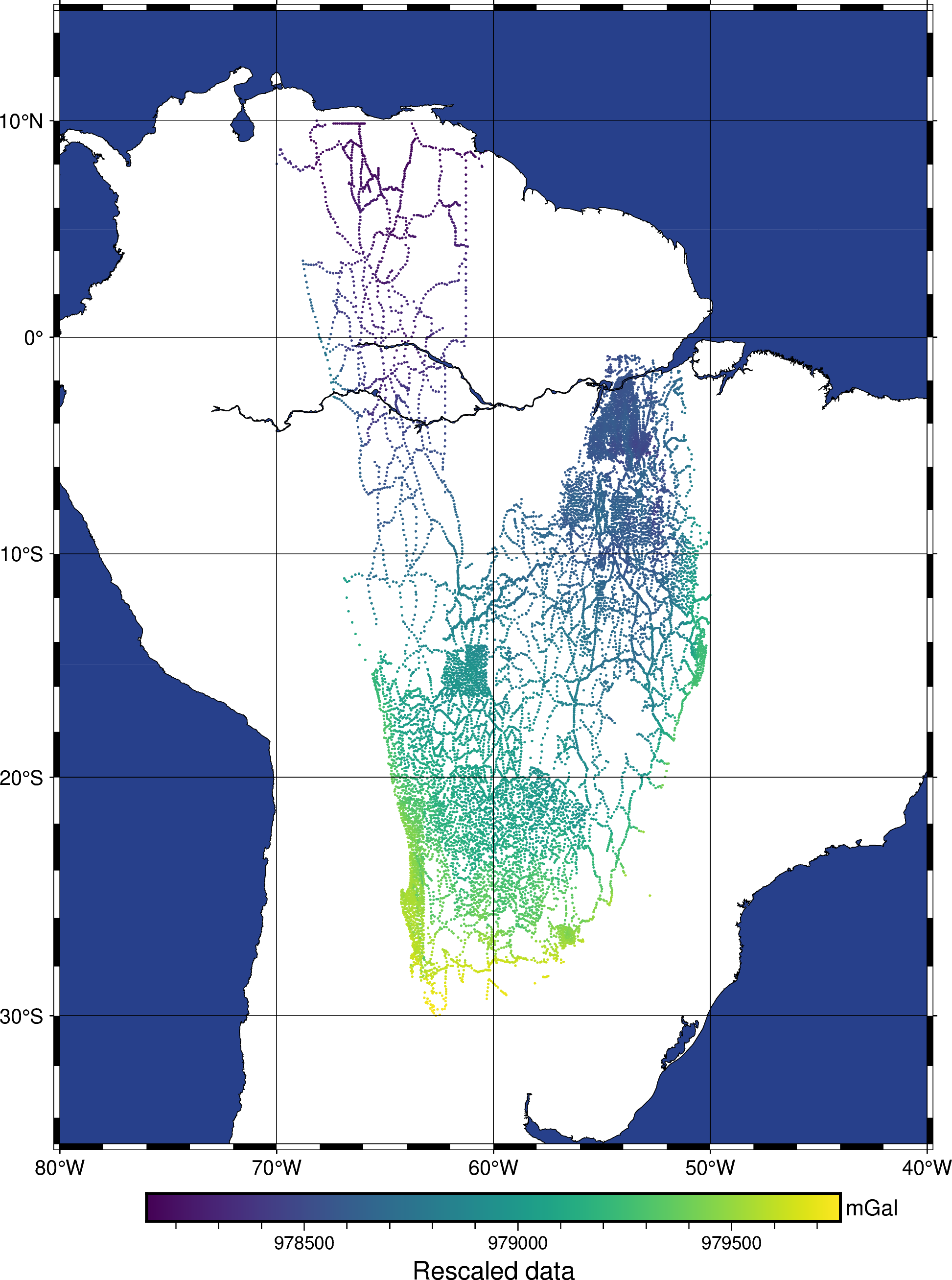
Notice how the general survey layout is retained, but the coordinates were translated to South America and stretch in latitude as desired.