6. Calculate data averages in blocks#

Point or line data can often be oversampled, for example along flight lines or ship tracks, or unevenly sampled across the data region. This can be undesired for plotting or lead to biases in interpolation and other analyses. A safe way to reduce (downsample) the data without causing aliasing is to divide the data into blocks and then take the mean or other statistic of the points that fall inside each block. We’ll demonstrate how to do this with bordado.block_split and pandas.

import ensaio
import pyproj
import pygmt
import pandas as pd
import bordado as bd

First, let’s get some topography data that we can use for this example through ensaio.fetch_british_columbia_lidar:

fname = ensaio.fetch_british_columbia_lidar(version=1)
data = pd.read_csv(fname)
data

	longitude	latitude	elevation_m
0	-123.813753	49.460263	-0.67
1	-123.813725	49.460274	-0.96
2	-123.813764	49.460254	-0.78
3	-123.813744	49.460262	-0.61
4	-123.813737	49.460265	-0.62
...	...	...	...
829728	-123.807407	49.455007	-1.24
829729	-123.807410	49.454995	-1.25
829730	-123.807416	49.454980	-1.19
829731	-123.807428	49.454966	-1.21
829732	-123.807432	49.454963	-1.20

829733 rows × 3 columns

This is a LIDAR dataset from a few islands in British Columbia, Canada. Let’s use bordado.get_region and bordado.pad_region to extract the data bounding box and pad it a little. This will be useful to make plots of the data without having the plot margins directly touching the data.

region = bd.pad_region(
    bd.get_region((data.longitude, data.latitude)),
    pad=(5 / 3600, 3 / 3600),
)
print(region)

(-123.82038848888888, -123.80540841111112, 49.45199186666667, 49.46111413333333)

Let’s plot the data with pygmt to see what we’ve got:

fig = pygmt.Figure()
pygmt.makecpt(
    cmap="viridis",
    series=[data.elevation_m.min(), data.elevation_m.max()],
)
fig.plot(
    x=data.longitude,
    y=data.latitude,
    fill=data.elevation_m,
    cmap=True,
    style="c0.01c",
    projection="M15c",
    region=region,
    frame="afg",
)
fig.colorbar(frame=["af+lOriginal topography", "y+lm"])
fig.show()

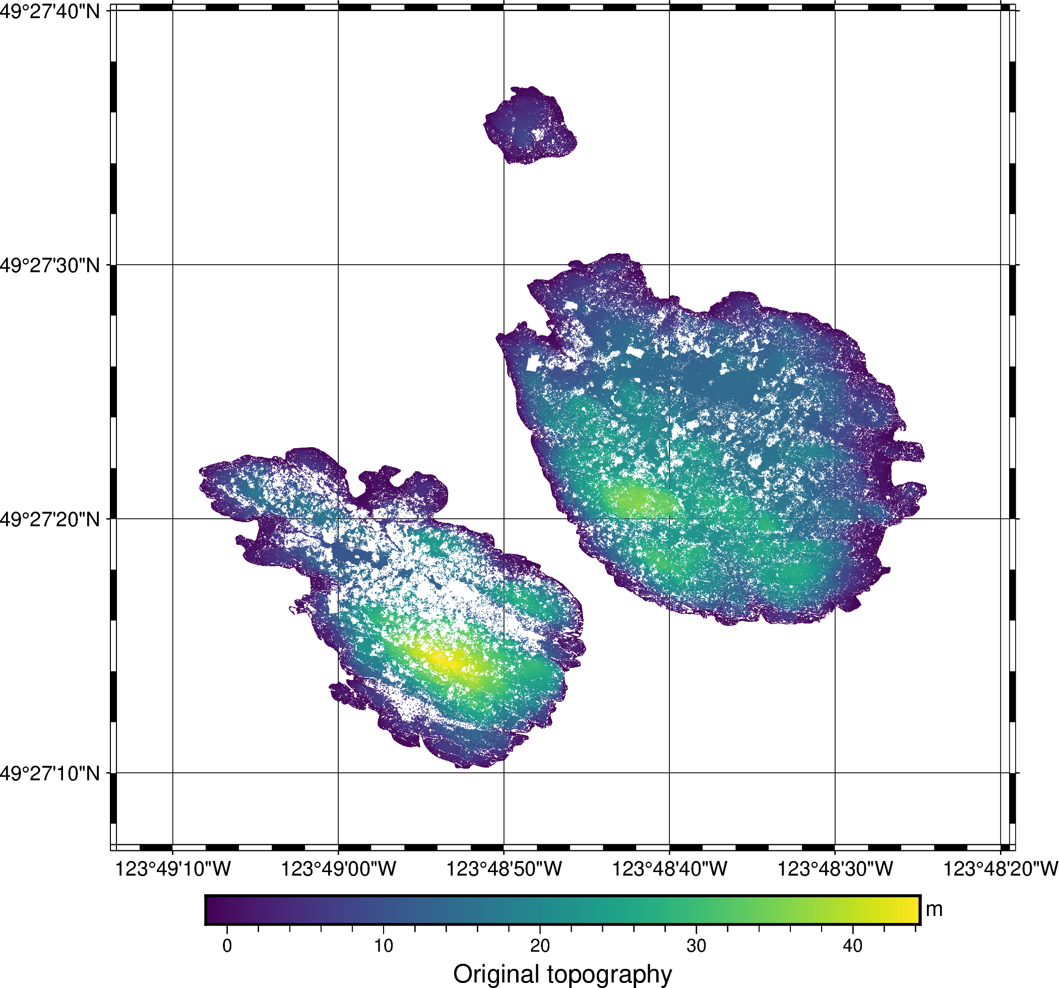
Notice that the sampling is not uniform, with areas of denser sampling and areas with no points at all.

The dataset is in geodetic longitude and latitude coordinates so we should first project it so we can use the regular Cartesian distance calculations in block_split:

projection = pyproj.Proj(proj="merc", lat_ts=data.latitude.mean())
easting, northing = projection(data.longitude, data.latitude)

Now we can divide the data into 2 meter blocks. The labels variable contains the index of the block to which each point belongs.

block_coordinates, labels = bd.block_split(
    coordinates=(easting, northing),
    block_size = 2,
)
data["block_id"] = labels
data

	longitude	latitude	elevation_m	block_id
0	-123.813753	49.460263	-0.67	183178
1	-123.813725	49.460274	-0.96	183179
2	-123.813764	49.460254	-0.78	182735
3	-123.813744	49.460262	-0.61	182736
4	-123.813737	49.460265	-0.62	183178
...	...	...	...	...
829728	-123.807407	49.455007	-1.24	53901
829729	-123.807410	49.454995	-1.25	53459
829730	-123.807416	49.454980	-1.19	53017
829731	-123.807428	49.454966	-1.21	53017
829732	-123.807432	49.454963	-1.20	52575

829733 rows × 4 columns

Our dataset now contains the block indices (IDs) for each point. To do a reduction operation (like mean, median, standard deviation, sum, etc), we can use the pandas.DataFrame.groupby method:

block_data = data.groupby("block_id").mean()
block_data

	longitude	latitude	elevation_m
block_id
155	-123.814695	49.452839	-1.025000
156	-123.814677	49.452836	-0.687692
157	-123.814654	49.452837	-0.262667
158	-123.814625	49.452836	-0.527143
159	-123.814594	49.452836	-0.517500
...	...	...	...
183188	-123.813461	49.460268	-1.058182
183189	-123.813437	49.460271	-0.916400
183190	-123.813410	49.460271	-0.952000
183191	-123.813386	49.460269	-0.964545
183192	-123.813363	49.460266	-1.190000

62928 rows × 3 columns

This new dataset has the mean longitude, latitude, and elevation per 2 meter block. The reduced dataset looks like this:

fig = pygmt.Figure()
pygmt.makecpt(
    cmap="viridis",
    series=[data.elevation_m.min(), data.elevation_m.max()],
)
fig.plot(
    x=block_data.longitude,
    y=block_data.latitude,
    fill=block_data.elevation_m,
    cmap=True,
    style="c0.01c",
    projection="M15c",
    region=region,
    frame="afg",
)
fig.colorbar(frame=["af+lBlock average topography", "y+lm"])
fig.show()

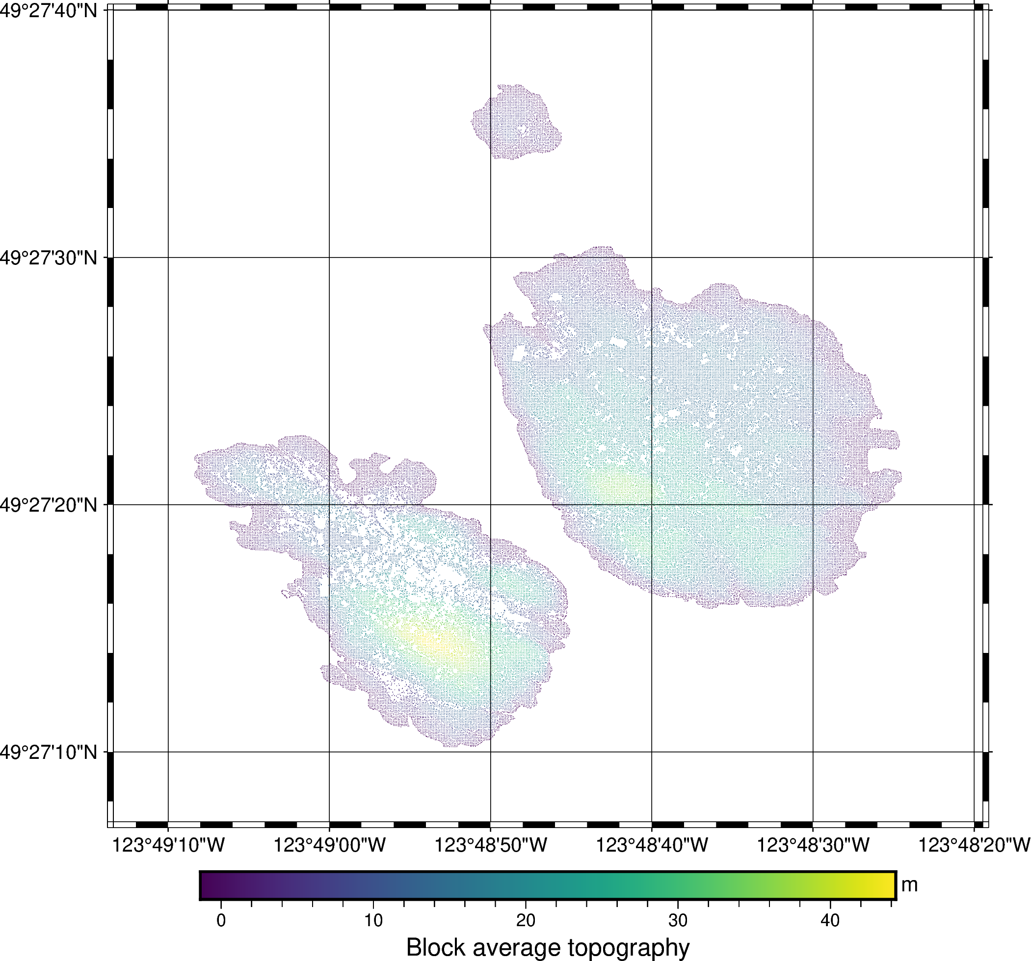
Notice that now the points are more uniformly spaced and there are no areas with much higher point density.