5. Splitting points into blocks#
Beyond generating values for coordinates, Bordado can also operate on them in a few useful ways. One category of this is splitting points spatially by segmenting them into blocks or windows. Functions bordado.block_split, bordado.expanding_window, bordado.rolling_window, and bordado.rolling_window_spherical are designed for this. This tutorial will teach you how to use them.
import bordado as bd
import numpy as np
import matplotlib.pyplot as plt
import pygmt
See also
We’ll use random data in these examples
generated by bordado.random_coordinates and
bordado.random_coordinates_spherical. See
“Random coordinates” to learn how to use them.
All of these segmentation functions generate arrays that can be used to index the coordinate arrays instead of actually doing any of the indexing themselves. This makes them more flexible to combine with other spatial operations that you may need.
5.1. Non-overlapping spatial blocks#
Bordado has function bordado.block_split that can provide indices for
segmenting coordinate arrays according to spatial blocks.
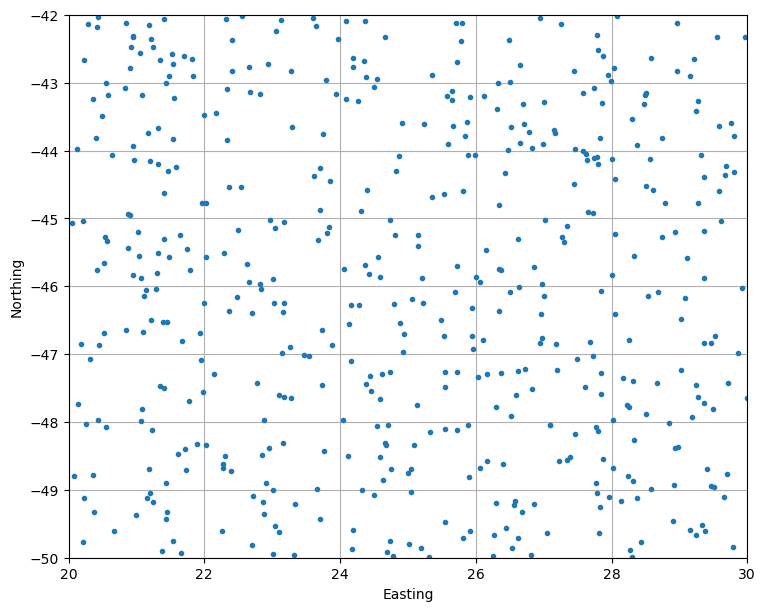
For this example, let’s make some random coordinates with
bordado.random_coordinates:
region = (20, 30, -50, -42)
coordinates = bd.random_coordinates(region, size=500, random_seed=42)

fig, ax = plt.subplots(1, 1, figsize=(8, 6), layout="constrained")
ax.plot(*coordinates, ".")
ax.set_aspect("equal")
ax.set_xlim(*region[:2])
ax.set_ylim(*region[2:])
ax.set_xlabel("Easting")
ax.set_ylabel("Northing")
ax.grid()
plt.show()
Then we can use block_split to get the indexers that split
these points into evenly sized blocks:
block_coordinates, labels = bd.block_split(coordinates, block_size=2)
print(labels)
[13 17 19 13 10 19  8 18  5  2  1 19  3  9  7  1  7 10  4 18 18  6  4 14
  3  5 17 15 15  8 13 14  6 11  2  0 10  2  1 18 17 14 18 16  4  9  6  1
 18  5  5  0  3 18  3  3  7  7 10  5  3  2 17 13 13 12 17  1  5 12  6 17
  9 16 15 11 16 13 17  8  8 12  4  5 15 10  3  7  0  2 15  8  7 11  1  8
 11 10 15 14  9 18 16 14 18 18 17  1 10  9 12 10 16 17  5 14 18  8  2  3
 17  8 15  7 15  7 16  0 10 17 15 19  2  6  2  0 14 12 18 15 12 17  4  2
 12 16  1 12 12  0  9 19 10  2 15  8 16  8 13  8  5 19  1  0  7 11 19 19
  6  9  1 12 16 14 10  5 17  9  4  8  4  4  2  6 13  8  6 15 18 11  9 16
  0  9 15 10 12 14 10  6  3  9  2 15  5 11 15 18  5  7 18 12 15 19 18  3
 10  0 14 16 11  7  3 19  1  4  0  2  8 10  5  2  4  7  4 14  2  8  5  5
  4  3 16  2 13  9  8  7 16 17  8  9  2  6 11  3  9 15  0  7 10  4  1  0
 19  0  1  0  0 10  0 10 10 17  3 16 11  2 19 19  5 15  6 11 17  7 15  6
 17 10  4  5  9  0  4  9  4  4 13 13 13  5 17 12  4  2 11  3 11 15  2  2
 16 11  1 16 16 13 11  9  4 12  6 12 19  3 14  2 18  6 13 10  8 14 10 13
 15 18  5 14  0 19 14  7  3 18  9 11  2 15  3  0 17 17  2  7 13 18  7 12
 14 10 15 10  3 17 18 18  1  4 13  1 16  6 10 15  9  7 11 13  7 14 18  7
  1  9  8  4  0 14  8 15  2  3 15 17  9  1  2 12  6  9  3  5 19 14  6  4
  5  9 18 18 15 19 15 16  0  3  5 14  3 15 10 10  3  9  1 19 10 14  9  8
  8 19 15  0 15  2 18  3  9 15  3  5  6  3 14 18 15  8 10  4  3  0 15 15
 19 12  8 13 12  5  4  1 17  8 18  4 10  2  7  2  0 15  6 11  7  8 13  2
 17 16 12  6  0 17  7  1  7 17 13 18 18  1 18  7 12  3 16  7]
The labels are the number of the block to which each point belongs. For example, these are the coordinates of the points that fall inside block 1:
block1 = tuple(c[labels == 1] for c in coordinates)

print("Coordinates of block 1:")
for i, c in enumerate(block1):
    print(f"coordinate {i}:\n{c}\n")
Coordinates of block 1:
coordinate 0:
[23.70798024 22.27238722 22.26909349 22.88328104 23.03950098 23.01512089
 22.72241562 23.31568997 22.30213991 22.90917838 22.86446227 23.10334674
 22.84720082 23.6639245  23.33637758 22.70534941 23.76359473 22.95359025
 22.38552821 23.01342633 22.25592868 23.16214152]

coordinate 1:
[-49.42352682 -48.61604444 -48.67274506 -49.35960573 -49.53513215
 -49.94148435 -49.08716743 -49.963999   -48.49925054 -48.90542978
 -49.17597853 -49.62100784 -48.4934242  -48.9847202  -49.20110018
 -49.81487924 -48.42606255 -48.38329519 -48.7175038  -48.99468918
 -49.59914648 -48.30436311]
The block_coordinates is a tuple with the coordinates of the center of each
block:
for c in block_coordinates:
    print(f"block coordinate {i}:\n{c}\n")
block coordinate 1:
[[21.04797324 23.03532303 25.02267282 27.01002262 28.99737241]
 [21.04797324 23.03532303 25.02267282 27.01002262 28.99737241]
 [21.04797324 23.03532303 25.02267282 27.01002262 28.99737241]
 [21.04797324 23.03532303 25.02267282 27.01002262 28.99737241]]

block coordinate 1:
[[-48.99262519 -48.99262519 -48.99262519 -48.99262519 -48.99262519]
 [-46.99760458 -46.99760458 -46.99760458 -46.99760458 -46.99760458]
 [-45.00258396 -45.00258396 -45.00258396 -45.00258396 -45.00258396]
 [-43.00756335 -43.00756335 -43.00756335 -43.00756335 -43.00756335]]
Tip
The keen-eyed among you might have noticed that the coordinates of the block
centers are not spaced by 2 (the block size). This is because by default
block_split extracts the region that is divided into blocks
from the input data, which are random and there are no points exactly on the
region boundaries. You can pass a region argument to make this be exact
or pass adjust="region"" to keep the block size fixed even if the region
is not passed.
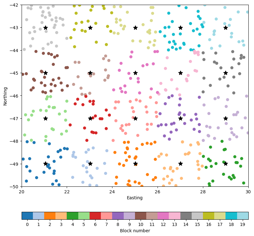
Let’s use matplotlib to plot this so we can understand it better.
We’ll plot the block centers as stars and a scatter of the points colored
according to which block they belong:
fig, ax = plt.subplots(1, 1, figsize=(8, 8), layout="constrained")
ax.plot(*block_coordinates, "k*", markersize=10)
tmp = ax.scatter(*coordinates, c=labels, cmap="tab20")
cb_region = (-0.5, 0.5 + labels.max())
fig.colorbar(
    tmp,
    label="Block number",
    orientation="horizontal",
    aspect=30,
    boundaries=bd.line_coordinates(*cb_region, spacing=1),
    values=bd.line_coordinates(*cb_region, spacing=1, pixel_register=True),
    ticks=bd.line_coordinates(*cb_region, spacing=1, pixel_register=True),
)
ax.set_aspect("equal")
ax.set_xlim(*region[:2])
ax.set_ylim(*region[2:])
ax.set_xlabel("Easting")
ax.set_ylabel("Northing")
plt.show()
The indexing is useful for calculating things like block means and other statistics. For example, we find out the number of points in each block like so:
points_per_block = [coordinates[0][labels == i].size for i in range(labels.max() + 1)]

print(points_per_block)
[25, 22, 30, 29, 25, 24, 20, 27, 26, 26, 30, 18, 21, 21, 22, 36, 21, 26, 31, 20]
5.2. Splitting into overlapping (rolling) windows#
In case we split points into blocks, but we want the blocks to overlap, the
operation is called a rolling window. Bordado implements this operation in
function bordado.rolling_window.
This is how we use it in the dataset we generated above with windows of size 4
and with a 50% overlap between adjacent windows:
window_coordinates, indices = bd.rolling_window(
    coordinates, window_size=4, overlap=0.5,
)
The window_coordinates is a tuple of coordinate arrays corresponding to the
center of each window. It will have the same number of arrays as coordinates
and works in any number of dimensions.
for c in window_coordinates:
    print(f"window coordinate {i}:\n{c}\n")
window coordinate 1:
[[22.05429834 24.03321466 26.01213098 27.9910473 ]
 [22.05429834 24.03321466 26.01213098 27.9910473 ]
 [22.05429834 24.03321466 26.01213098 27.9910473 ]]

window coordinate 1:
[[-47.9901355  -47.9901355  -47.9901355  -47.9901355 ]
 [-46.00009427 -46.00009427 -46.00009427 -46.00009427]
 [-44.01005304 -44.01005304 -44.01005304 -44.01005304]]
Hint
Notice that the window size is adjusted here as well to fit the region
of the points. To prevent this from happening, either pass a region or
adjust="region" to rolling_window.
Like the block_coordinates above, the arrays have the number of dimensions
of the input coordinates (in this case, 2D).
The indices are a bit more complex than the labels from block_split. They are an array with the same shape as the window_coordinates:
print(window_coordinates[0].shape)
print(indices.shape)
(3, 4)
(3, 4)
Each element of the indices array corresponds to a window and is an index for selecting points that fall inside that window. For example, this is the index for the first window:
print(indices[0, 0])
(array([  8,  10,  15,  21,  25,  32,  35,  38,  46,  47,  49,  50,  51,
        59,  67,  68,  70,  83,  88,  94, 107, 114, 127, 133, 135, 146,
       149, 160, 162, 163, 168, 170, 175, 183, 186, 192, 199, 204, 208,
       217, 224, 226, 230, 238, 239, 253, 258, 262, 263, 265, 266, 267,
       268, 270, 280, 282, 287, 291, 293, 301, 314, 322, 329, 338, 340,
       351, 368, 371, 373, 384, 388, 397, 400, 403, 406, 408, 416, 418,
       426, 435, 443, 444, 453, 461, 463, 470, 472, 474, 483, 484, 487,
       493]),)
Tip
Notice that it’s a tuple with one index array. This is because our
coordinates are 1D arrays. If they were 2D arrays (for example, if they
were a regular grid), then indices[0, 0] would be a tuple with 2 index
arrays.
We can select the points that fall inside the first window like so:
window = [c[indices[0, 0]] for c in coordinates]

print("Coordinates of window 0, 0:")
for i, c in enumerate(window):
    print(f"coordinate {i}:\n{c}\n")
Coordinates of window 0, 0:
coordinate 0:
[21.28113633 23.70798024 22.27238722 23.54525968 21.94638708 23.25825358
 21.89471359 22.26909349 23.87478379 22.88328104 21.39752484 21.99908202
 20.0736227  21.14530074 23.03950098 20.30817835 22.14584673 21.6697292
 21.61271779 23.01512089 22.72241562 21.76772783 21.44524189 23.46869805
 20.22803871 23.31568997 20.2161208  21.07740946 22.30213991 20.37412556
 23.17138893 22.90917838 20.44910619 23.15929052 23.73657729 21.22757932
 23.10323673 20.13936288 21.21832505 21.23753804 22.86446227 20.24859491
 21.40339597 20.17836784 21.09143997 22.47839563 20.66558857 23.10334674
 21.43871933 21.65531723 22.84720082 21.53613395 21.15490064 20.55395409
 20.43475062 22.36744871 23.73614138 20.51961866 20.99113142 21.34552208
 23.6639245  23.28361205 22.88155614 20.84493219 21.3740793  21.71291304
 23.33637758 22.70534941 23.1443998  23.76359473 21.18478577 22.95359025
 23.01927391 21.10588411 22.83908438 21.06419532 21.43021875 21.98204227
 22.38552821 22.01782111 21.93041491 22.70758751 21.73127846 21.45130255
 23.01342633 24.04034391 21.19217526 22.78075546 23.17040911 20.36059834
 22.25592868 23.16214152]

coordinate 1:
[-46.04686683 -49.42352682 -48.61604444 -47.02190741 -47.08064511
 -46.89726644 -48.32753873 -48.67274506 -46.85941827 -49.35960573
 -46.52976778 -46.24538453 -48.79461621 -46.05368019 -49.53513215
 -47.06713292 -47.29234813 -46.81157995 -48.46717592 -49.94148435
 -49.08716743 -47.69417404 -49.32144582 -47.01838127 -49.12574167
 -49.963999   -49.76314169 -47.80139959 -48.49925054 -49.32150727
 -47.62910354 -48.90542978 -46.86104726 -46.37376067 -46.63694583
 -48.11922306 -47.60493367 -47.73402453 -46.49290993 -49.18484674
 -49.17597853 -48.03146711 -47.49944041 -46.84699378 -46.66712294
 -46.1610928  -49.61144568 -49.62100784 -48.89435703 -49.92592175
 -48.4934242  -49.7497319  -49.11496426 -48.06688873 -47.96589213
 -46.36434056 -47.45280706 -46.68779125 -49.37513286 -47.46277463
 -48.9847202  -47.64195845 -47.97068395 -46.6458209  -49.90024098
 -48.40366406 -49.20110018 -49.81487924 -46.98284256 -48.42606255
 -48.697028   -48.38329519 -46.25266687 -46.14806928 -46.03594755
 -47.98050968 -49.42542288 -47.56426779 -48.7175038  -48.34549178
 -46.69145655 -46.4011256  -48.7099675  -46.52349532 -48.99468918
 -47.97452315 -49.04837351 -47.42773607 -46.24992562 -48.77698302
 -49.59914648 -48.30436311]
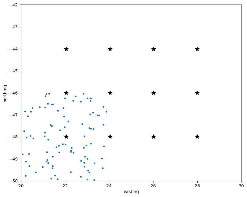
And then we can plot the window centers and the points of the first window:
fig, ax = plt.subplots(1, 1, figsize=(8, 7), layout="constrained")
ax.plot(*window, ".")
ax.plot(*window_coordinates, "k*", markersize=10)
ax.set_aspect("equal")
ax.set_xlim(*region[:2])
ax.set_ylim(*region[2:])
ax.set_xlabel("easting")
ax.set_ylabel("northing")
plt.show()
We can do this for other windows as well, like the one to the right of 0, 0:
window = [c[indices[0, 1]] for c in coordinates]

fig, ax = plt.subplots(1, 1, figsize=(8, 7), layout="constrained")
ax.plot(*window, ".")
ax.plot(*window_coordinates, "k*", markersize=10)
ax.set_aspect("equal")
ax.set_xlim(*region[:2])
ax.set_ylim(*region[2:])
ax.set_xlabel("Easting")
ax.set_ylabel("Northing")
plt.show()
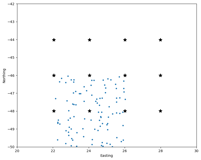
Notice that there is overlap and 50% (the chosen overlap) of the points
belong to both windows.
5.3. Spatial blocks on the sphere#
The splitting strategies we’ve seen so far won’t work well for geographic data since blocks and windows
will get smaller and smaller towards the poles because of the convergence of
meridians.
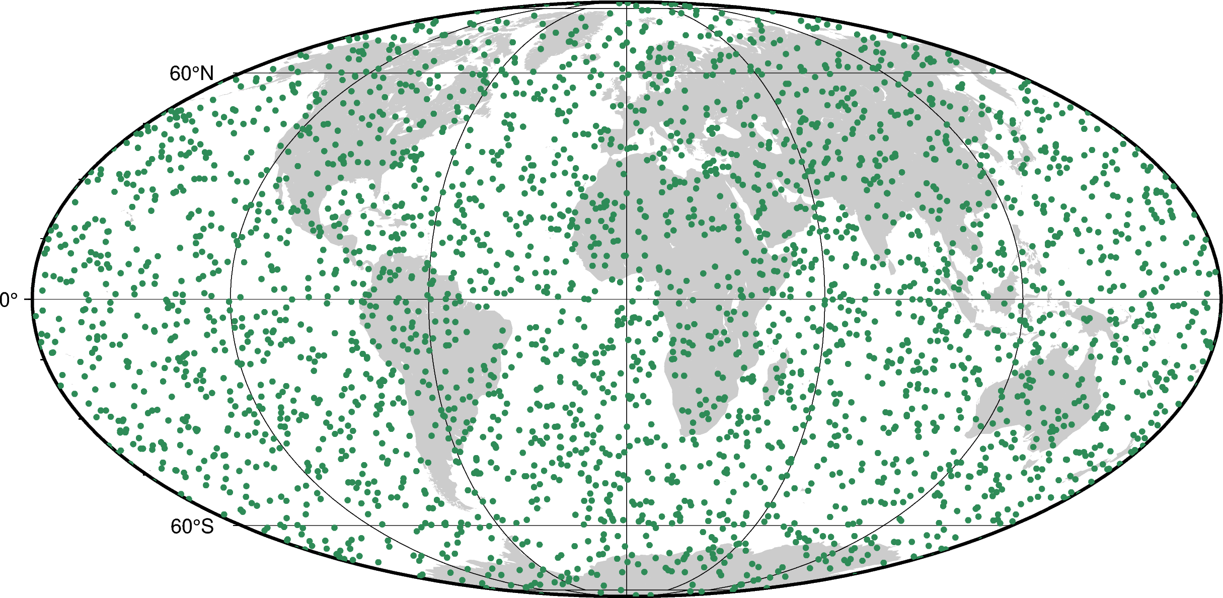
To demonstrate this, let’s first make some random points that are uniformly distributed on the sphere with bordado.random_coordinates_spherical:
region = (0, 360, -90, 90)  # W, E, S, N in degrees
coordinates = bd.random_coordinates_spherical(region, size=3000)

fig = pygmt.Figure()
fig.coast(land="#cccccc", region="g", projection="W0/20c", frame="afg")
fig.plot(x=coordinates[0], y=coordinates[1], style="c0.1c", fill="seagreen")
fig.show()
Now we can split them into 30° blocks in both longitude and latitude using the
standard bordado.block_split:
block_coordinates, labels = bd.block_split(coordinates, block_size=30)

fig = pygmt.Figure()
fig.coast(land="#cccccc", region="g", projection="W0/20c")
fig.plot(
    x=coordinates[0],
    y=coordinates[1],
    style="c0.1c",
    fill=labels,
    cmap="gmt/categorical",
)
fig.plot(
    x=block_coordinates[0].ravel(),
    y=block_coordinates[1].ravel(),
    style="a0.5c",
    fill="black",
    frame="af",
)
fig.show()
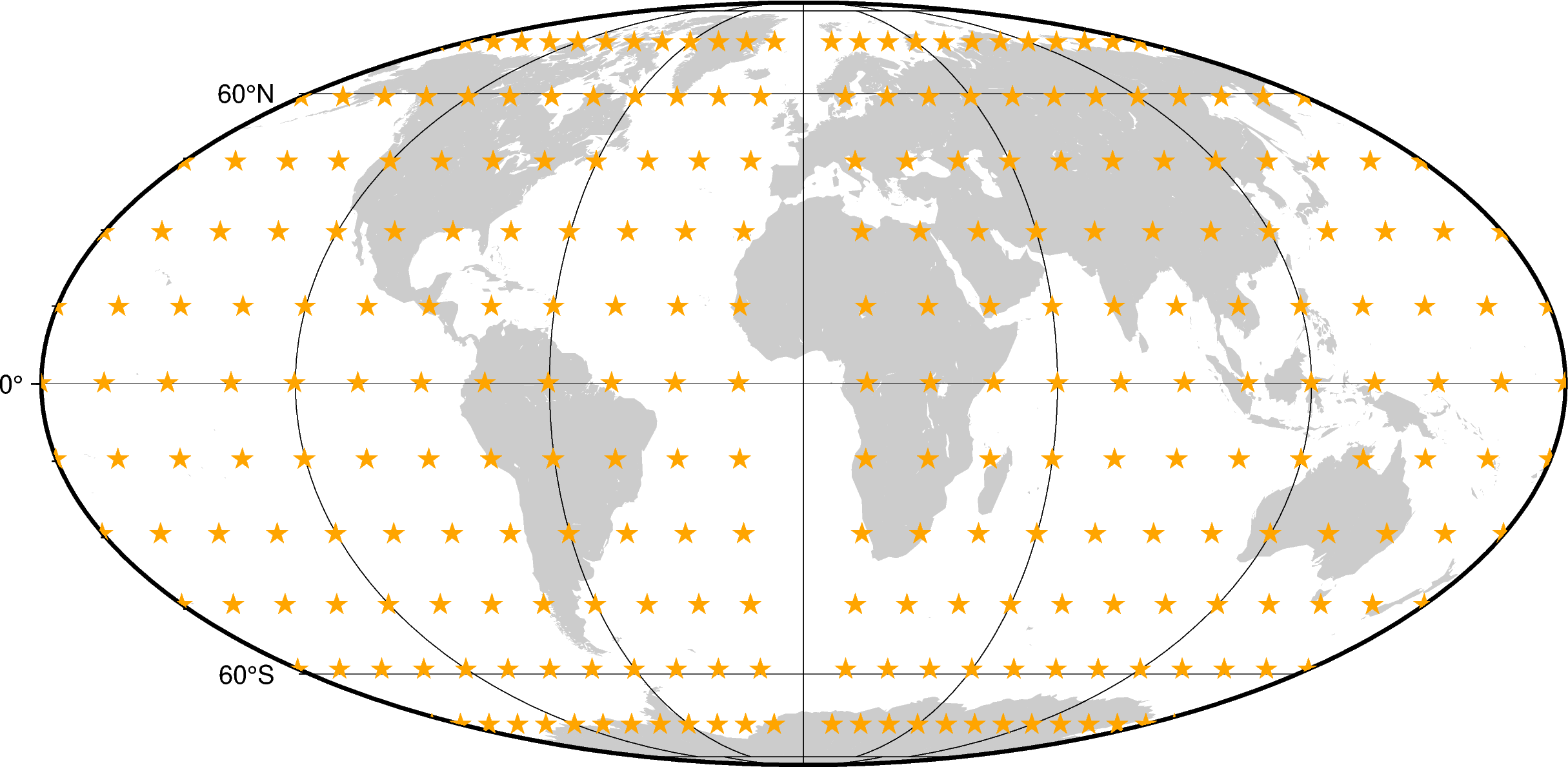
Notice that the blocks get closer together as we go from the equator to the poles. This means that the number of points in each block is not equal. Let’s calculate the number of points per block and plot that against the block latitude to illustrate:
points_per_block = [
    coordinates[0][labels == i].size
    for i in range(block_coordinates[0].size)
]
block_latitude = block_coordinates[1].ravel()

fig, ax = plt.subplots(1, 1, figsize=(8, 5), layout="constrained")
ax.plot(block_latitude, points_per_block, ".")
ax.set_xlabel("Block latitude")
ax.set_ylabel("Points per block")
ax.grid()
plt.show()
Remember that the points are evenly distributed on the sphere so we don’t expect any trend towards the poles. But what we see is exactly that. There are fewer points per block towards the poles.
To get around this, we can increase the longitudinal block size as a function of
the latitude to counteract the convergence of the meridians.
That’s what bordado.block_split_spherical does!
block_coordinates, labels = bd.block_split_spherical(
    coordinates, block_size=30,
)
print(labels)
[11 27 17 ... 25 26 2]
The output is very similar to the standard block_split. The
labels correspond to the index of the block to which that data point belongs.
But this time, the block coordinates will always be 1D arrays since they are not
regularly distributed:
print("Block longitudes:", block_coordinates[0])
print("Block latitudes:", block_coordinates[1])
Block longitudes: [ 45.01474014 134.99085331 224.96696647 314.94307964  20.02137537
  60.010759   100.00014263 139.98952626 179.97890989 219.96829352
 259.95767715 299.94706078 339.93644441  15.02270242  45.01474014
  75.00677786 104.99881558 134.99085331 164.98289103 194.97492875
 224.96696647 254.95900419 284.95104192 314.94307964 344.93511736
  15.02270242  45.01474014  75.00677786 104.99881558 134.99085331
 164.98289103 194.97492875 224.96696647 254.95900419 284.95104192
 314.94307964 344.93511736  20.02137537  60.010759   100.00014263
 139.98952626 179.97890989 219.96829352 259.95767715 299.94706078
 339.93644441  60.010759   179.97890989 299.94706078]
Block latitudes: [-71.87051384 -71.87051384 -71.87051384 -71.87051384 -42.83420105
 -42.83420105 -42.83420105 -42.83420105 -42.83420105 -42.83420105
 -42.83420105 -42.83420105 -42.83420105 -13.79788825 -13.79788825
 -13.79788825 -13.79788825 -13.79788825 -13.79788825 -13.79788825
 -13.79788825 -13.79788825 -13.79788825 -13.79788825 -13.79788825
  15.23842455  15.23842455  15.23842455  15.23842455  15.23842455
  15.23842455  15.23842455  15.23842455  15.23842455  15.23842455
  15.23842455  15.23842455  44.27473735  44.27473735  44.27473735
  44.27473735  44.27473735  44.27473735  44.27473735  44.27473735
  44.27473735  73.31105014  73.31105014  73.31105014]
Note
Notice that the latitudinal spacing between block centers isn’t exactly
30°. This is because the region that is split into blocks is inferred from
the coordinates (using bordado.get_region) and the block size
ended up getting adjusted to fit the region. To get exactly global coverage
or a particular region, pass the region argument.
Plotting the points and their labels for comparison yields:
fig = pygmt.Figure()
fig.coast(land="#cccccc", region="g", projection="W0/20c")
fig.plot(
    x=coordinates[0],
    y=coordinates[1],
    style="c0.1c",
    fill=labels,
    cmap="gmt/categorical",
)
fig.plot(
    x=block_coordinates[0],
    y=block_coordinates[1],
    style="a0.5c",
    fill="black",
    frame="af",
)
fig.show()
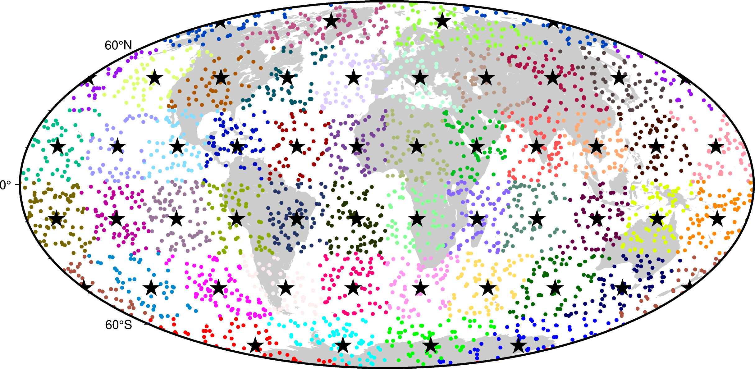
We can see that the block coordinates are no longer converging towards the poles and that there are fewer blocks than the standard version. To help quantify this, we can do the same points-per-block calculation from earlier and compare both methods:
points_per_block_spherical = [
    coordinates[0][labels == i].size
    for i in range(block_coordinates[0].size)
]
block_latitude_spherical = block_coordinates[1].ravel()

fig, ax = plt.subplots(1, 1, figsize=(8, 5), layout="constrained")
ax.plot(block_latitude, points_per_block, ".", label="Regular")
ax.plot(
    block_latitude_spherical,
    points_per_block_spherical,
    "*",
    label="Spherical",
)
ax.set_xlabel("Block latitude")
ax.set_ylabel("Points per block")
ax.grid()
ax.legend()
plt.show()
Notice that the spherical version keeps the points per block relatively constant with latitude, which is what we wanted.
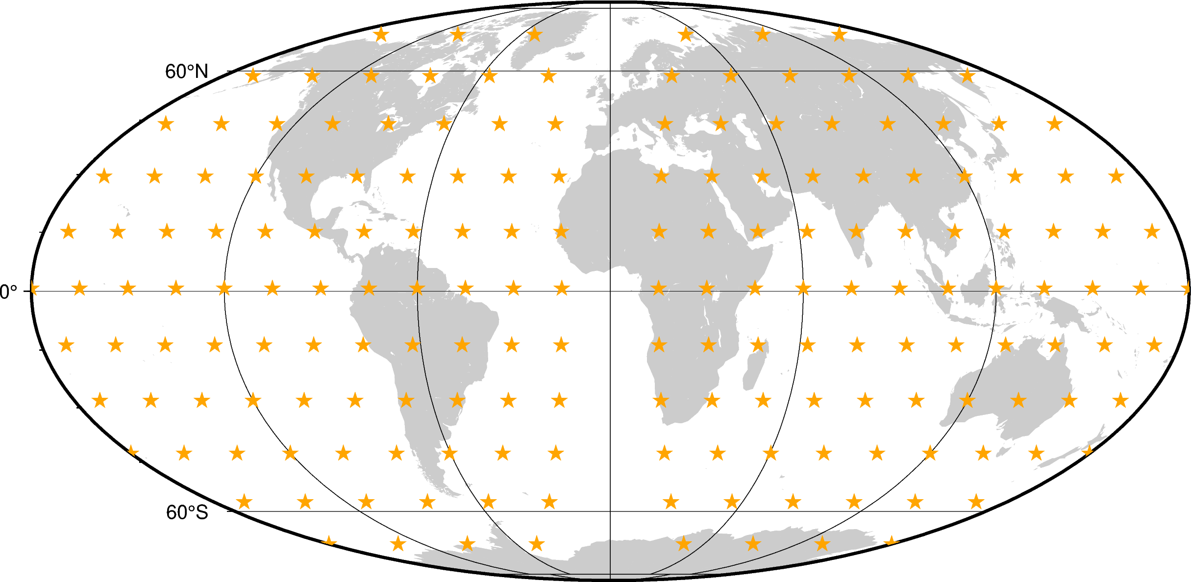
5.4. Rolling windows on the sphere#
The same logic from splitting into spherical blocks can be applied to the
rolling windows.
Let’s first split our random data into 30° windows with 50% overlap using the
standard rolling_window and plot the window centers:
window_coordinates, indices = bd.rolling_window(
    coordinates, window_size=30, overlap=0.5,
)

fig = pygmt.Figure()
fig.coast(land="#cccccc", region="g", projection="W0/20c", frame="afg")
fig.plot(
    x=window_coordinates[0].ravel(),
    y=window_coordinates[1].ravel(),
    style="a0.3c",
    fill="orange",
)
fig.show()
The window centers get closer as windows get smaller towards the poles. This can be a problem since windows towards the equator will likely contain more points, skewing any statistics or other math done on the data inside windows. There is also a gap at the 360° - 0° boundary since the function doesn’t know that it’s a periodic boundary.
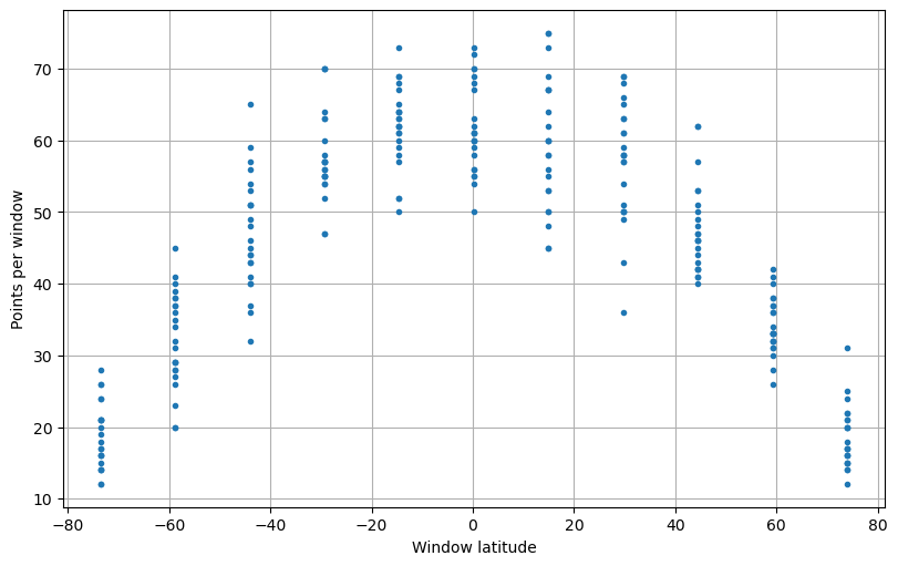
We can show this by calculating the number of points inside each window and plotting that as a function of the window center latitude:
points_per_window = [coordinates[0][i].size for i in indices.ravel()]
window_latitude = window_coordinates[1].ravel()

fig, ax = plt.subplots(1, 1, figsize=(8, 5), layout="constrained")
ax.plot(window_latitude, points_per_window, ".")
ax.set_xlabel("Window latitude")
ax.set_ylabel("Points per window")
ax.grid()
plt.show()
It’s clear from the plot above that there are fewer points inside windows at the poles, even though the distribution of points is uniform.
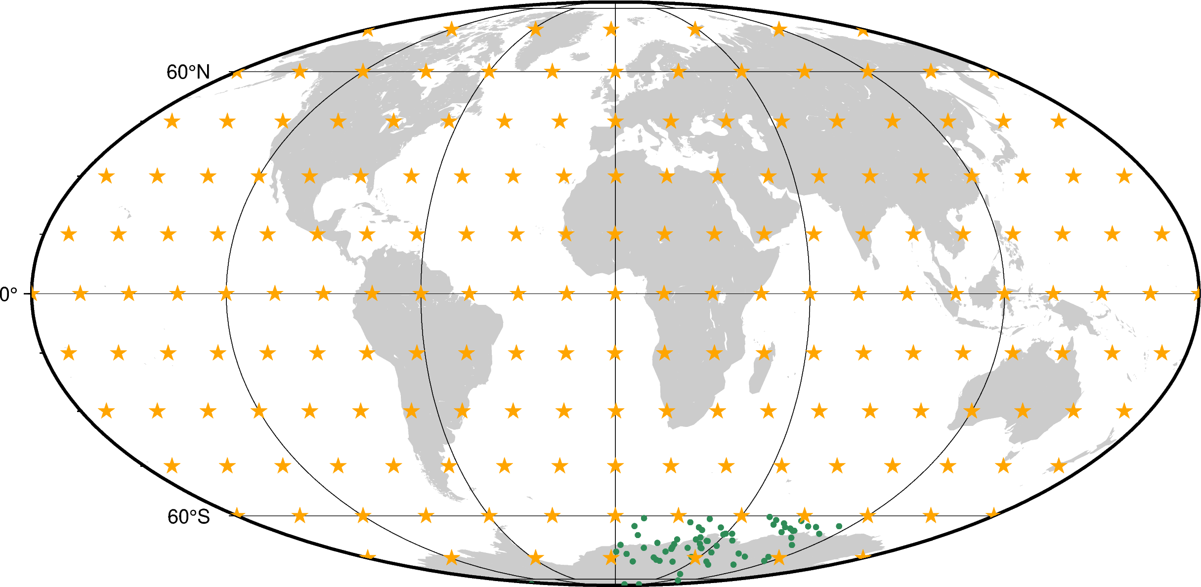
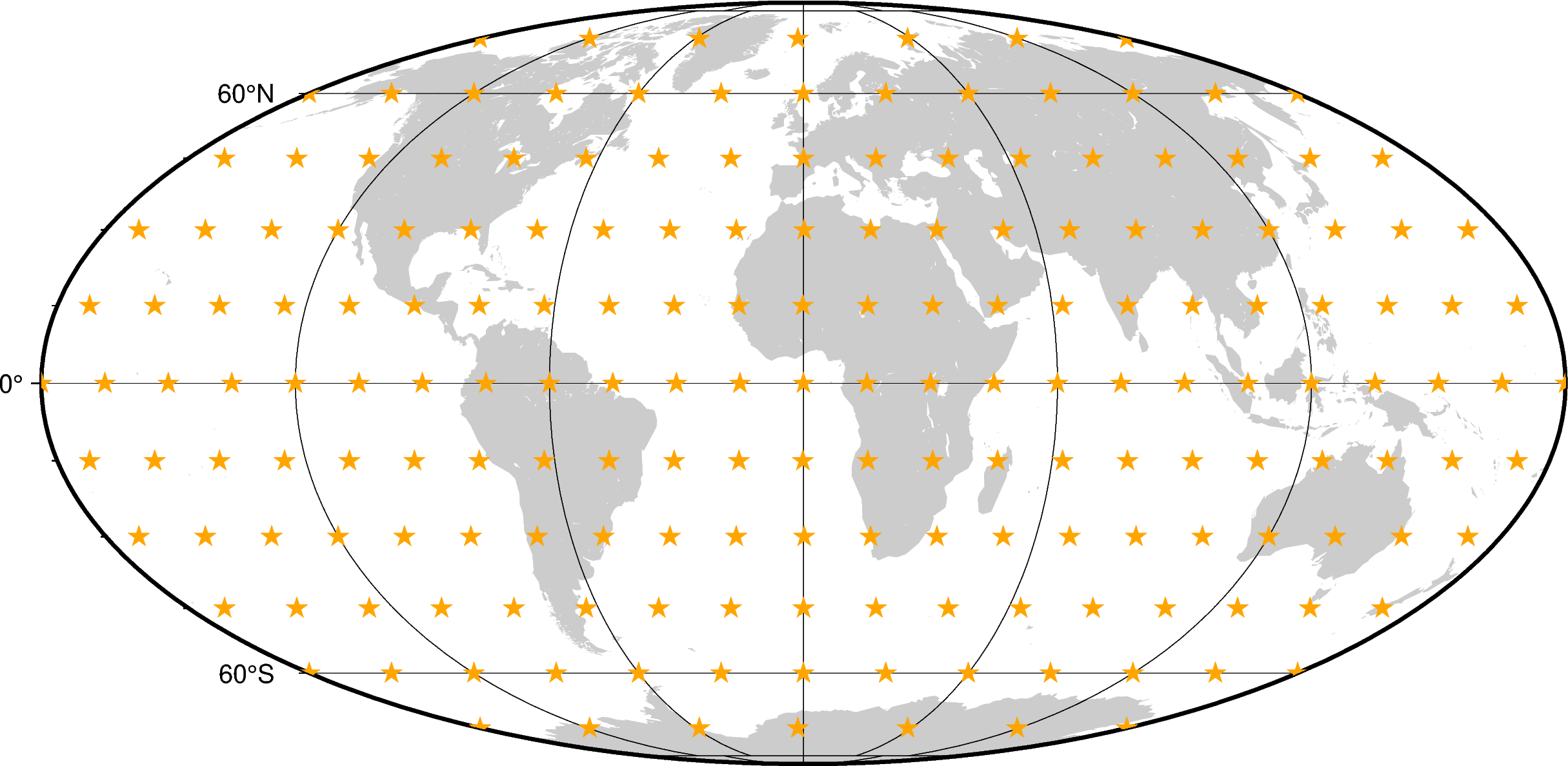
To get around this, use bordado.rolling_window_spherical:
window_coordinates, indices = bd.rolling_window_spherical(
    coordinates, window_size=30, overlap=0.5,
)

fig = pygmt.Figure()
fig.coast(land="#cccccc", region="g", projection="W0/20c", frame="afg")
fig.plot(
    x=window_coordinates[0].ravel(),
    y=window_coordinates[1].ravel(),
    style="a0.3c",
    fill="orange",
)
ax.set_title("Standard rolling windows")
fig.show()
Tip
The windows now don’t have a fixed 30° x 30° size to compensate for the
convergence of the meridians. This means that the window_size argument of
rolling_window_spherical refers to the latitudinal size of
the windows. The longitudinal size will vary depending on the latitude band
of the window.
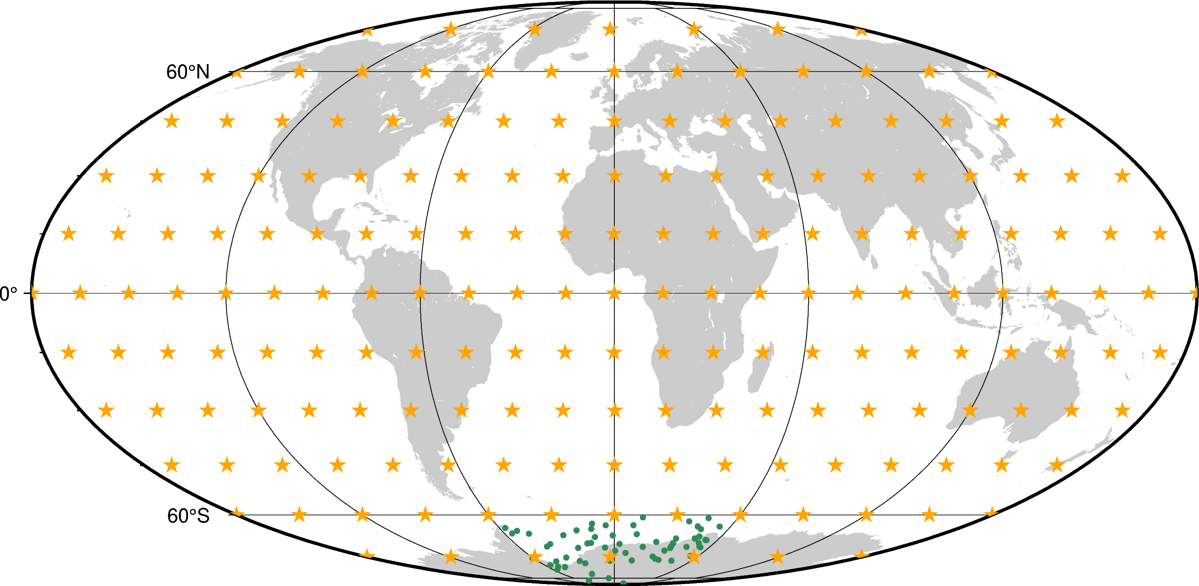
In this case, the window centers don’t get closer towards the poles. But there
is still the 360° - 0° gap. This happens because the region isn’t exactly
360° in longitude and so the code doesn’t know that it should wrap around the
globe. To get around this, we can specify the region argument with the full
range:
window_coordinates, indices = bd.rolling_window_spherical(
    coordinates, window_size=30, overlap=0.5, region=(0, 360, -90, 90),
)

fig = pygmt.Figure()
fig.coast(land="#cccccc", region="g", projection="W0/20c", frame="afg")
fig.plot(
    x=window_coordinates[0].ravel(),
    y=window_coordinates[1].ravel(),
    style="a0.3c",
    fill="orange",
)
fig.show()
This time, since the window centers aren’t on a regular grid anymore, both the
window_coordinates and indices are 1D arrays:
print(f"Coordinate shapes:", end=" ")
for c in window_coordinates:
    print(c.shape, end=" ")
print("\nIndices shape:", indices.shape)
Coordinate shapes: (182,) (182,)
Indices shape: (182,)
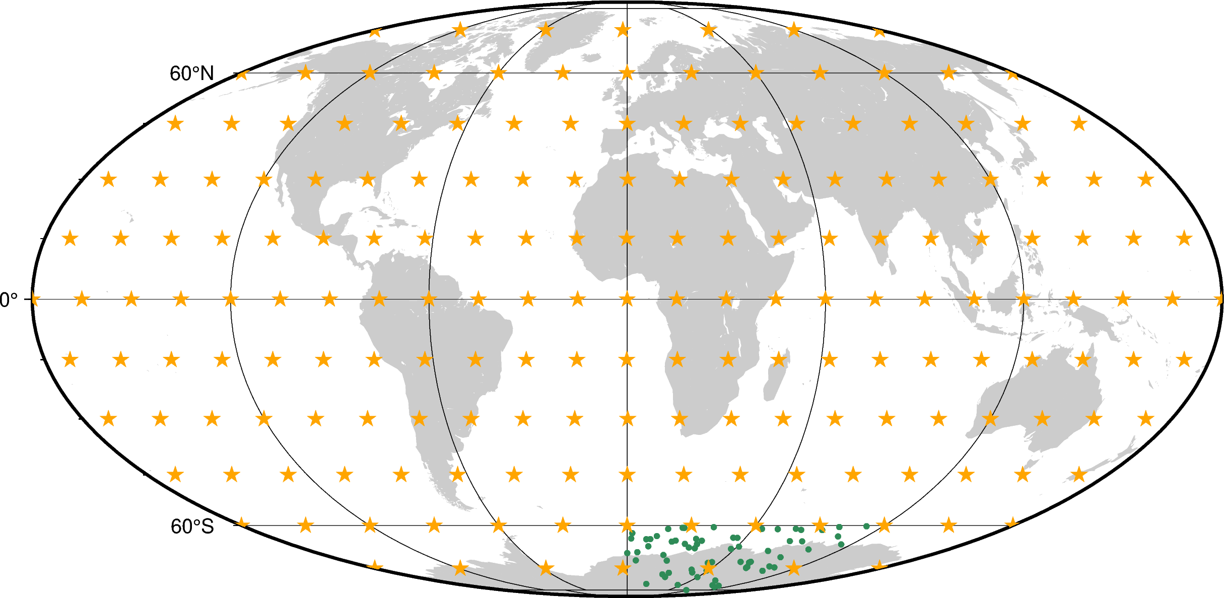
Let’s plot the points from some of the windows:
window = [c[indices[0]] for c in coordinates]

fig = pygmt.Figure()
fig.coast(land="#cccccc", region="g", projection="W0/20c", frame="afg")
fig.plot(
    x=window[0].ravel(), y=window[1].ravel(), style="c0.1c", fill="seagreen",
)
fig.plot(
    x=window_coordinates[0].ravel(),
    y=window_coordinates[1].ravel(),
    style="a0.3c",
    fill="orange",
)
fig.show()
window = [c[indices[5]] for c in coordinates]

fig = pygmt.Figure()
fig.coast(land="#cccccc", region="g", projection="W0/20c", frame="afg")
fig.plot(
    x=window[0].ravel(), y=window[1].ravel(), style="c0.1c", fill="seagreen",
)
fig.plot(
    x=window_coordinates[0].ravel(),
    y=window_coordinates[1].ravel(),
    style="a0.3c",
    fill="orange",
)
fig.show()
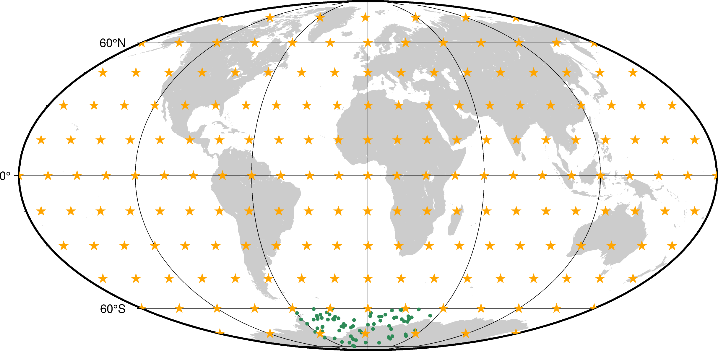
Note
Notice that there is an overlap between the two windows plotted above that crosses the 360° - 0° line.
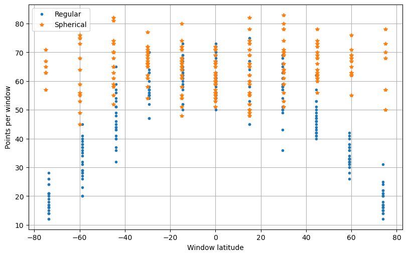
Making the same points per window calculation as before, we can check if it actually works:
points_per_window_spherical = [coordinates[0][i].size for i in indices.ravel()]
window_latitude_spherical = window_coordinates[1].ravel()

fig, ax = plt.subplots(1, 1, figsize=(8, 5), layout="constrained")
ax.plot(window_latitude, points_per_window, ".", label="Regular")
ax.plot(window_latitude_spherical, points_per_window_spherical, "*", label="Spherical")
ax.legend()
ax.set_xlabel("Window latitude")
ax.set_ylabel("Points per window")
ax.grid()
plt.show()
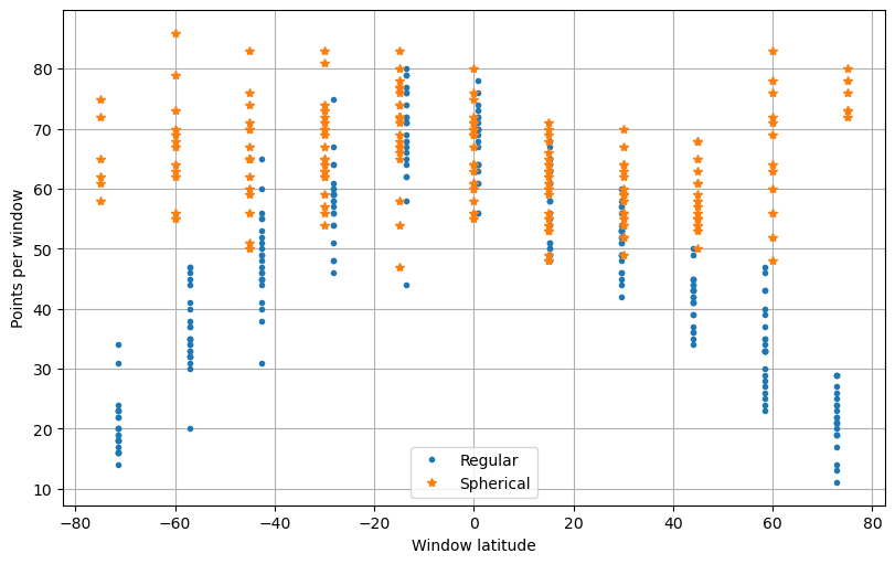
Now the distribution is much more uniform!
5.5. What’s next#
With this, we’ve finished our tutorial! To learn more about Bordado, take a look at the detailed documentation for each function in “List of functions and classes (API)” and examples of how to solve specific problems in “How To”.
Please remember to cite Bordado if you use it in a publication, thesis, report, etc. It helps us justify the effort that goes into making this package.
Have questions?
Please ask on any of the Fatiando a Terra community channels!