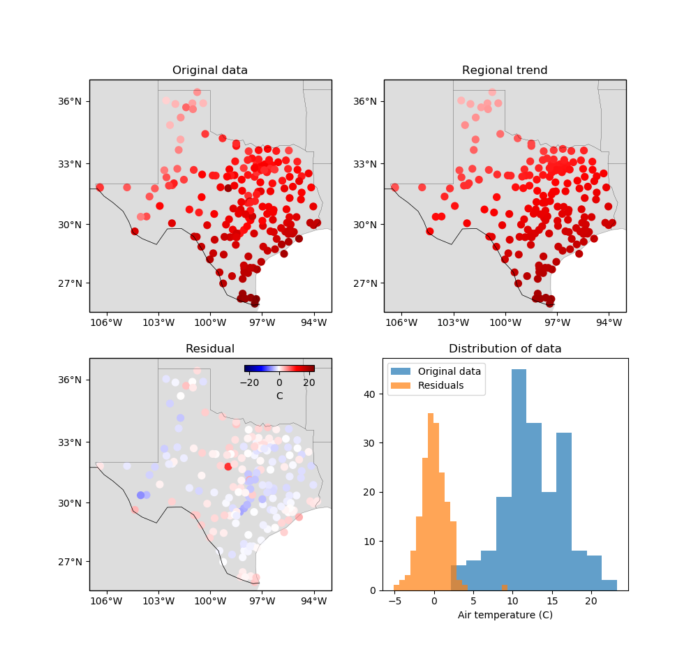
Polynomial trend

Verde offers the verde.Trend class to fit a 2D polynomial trend to your data. This can be useful for isolating a regional component of your data, for example, which is a common operation for gravity and magnetic data. Let’s look at how we can use Verde to remove the clear trend from our Texas temperature dataset (verde.datasets.fetch_texas_wind).

Out:

Original data:
  station_id  longitude  ...  wind_speed_east_knots  wind_speed_north_knots
0        0F2   -97.7756  ...               1.032920               -2.357185
1        11R   -96.3742  ...               1.692155                2.982564
2        2F5  -101.9018  ...              -1.110056               -0.311412
3        3T5   -96.9500  ...               1.695097                3.018448
4        5C1   -98.6946  ...               1.271400                1.090743

[5 rows x 6 columns]

Trend estimator: Trend(degree=1)

Updated DataFrame:
  station_id  longitude  latitude  ...  wind_speed_north_knots      trend  residual
0        0F2   -97.7756   33.6017  ...               -2.357185   9.067526  0.168585
1        11R   -96.3742   30.2189  ...                2.982564  14.727121 -0.512816
2        2F5  -101.9018   32.7479  ...               -0.311412   8.508071 -1.438626
3        3T5   -96.9500   29.9100  ...                3.018448  14.931638 -0.434877
4        5C1   -98.6946   29.7239  ...                1.090743  14.434636 -1.476303

[5 rows x 8 columns]
/home/travis/build/fatiando/verde/examples/trend.py:78: UserWarning: This figure includes Axes that are not compatible with tight_layout, so results might be incorrect.
  plt.tight_layout()
/home/travis/build/fatiando/verde/examples/trend.py:78: UserWarning: Tight layout not applied. The left and right margins cannot be made large enough to accommodate all axes decorations.
  plt.tight_layout()

import numpy as np
import matplotlib.pyplot as plt
import cartopy.crs as ccrs
import verde as vd

# Load the Texas wind and temperature data as a pandas.DataFrame
data = vd.datasets.fetch_texas_wind()
print("Original data:")
print(data.head())

# Fit a 1st degree 2D polynomial to the data
coordinates = (data.longitude, data.latitude)
trend = vd.Trend(degree=1).fit(coordinates, data.air_temperature_c)
print("\nTrend estimator:", trend)

# Add the estimated trend and the residual data to the DataFrame
data["trend"] = trend.predict(coordinates)
data["residual"] = data.air_temperature_c - data.trend
print("\nUpdated DataFrame:")
print(data.head())


# Make a function to plot the data using the same colorbar
def plot_data(column, i, title):
    "Plot the column from the DataFrame in the ith subplot"
    crs = ccrs.PlateCarree()
    ax = plt.subplot(2, 2, i, projection=ccrs.Mercator())
    ax.set_title(title)
    # Set vmin and vmax to the extremes of the original data
    maxabs = vd.maxabs(data.air_temperature_c)
    mappable = ax.scatter(
        data.longitude,
        data.latitude,
        c=data[column],
        s=50,
        cmap="seismic",
        vmin=-maxabs,
        vmax=maxabs,
        transform=crs,
    )
    # Set the proper ticks for a Cartopy map
    vd.datasets.setup_texas_wind_map(ax)
    return mappable


plt.figure(figsize=(10, 9.5))

# Plot the data fields and capture the mappable returned by scatter to use for
# the colorbar
mappable = plot_data("air_temperature_c", 1, "Original data")
plot_data("trend", 2, "Regional trend")
plot_data("residual", 3, "Residual")

# Make histograms of the data and the residuals to show that the trend was
# removed
ax = plt.subplot(2, 2, 4)
ax.set_title("Distribution of data")
ax.hist(data.air_temperature_c, bins="auto", alpha=0.7, label="Original data")
ax.hist(data.residual, bins="auto", alpha=0.7, label="Residuals")
ax.legend()
ax.set_xlabel("Air temperature (C)")

# Add a single colorbar on top of the histogram plot where there is some space
cax = plt.axes((0.35, 0.44, 0.10, 0.01))
cb = plt.colorbar(mappable, cax=cax, orientation="horizontal",)
cb.set_label("C")

plt.tight_layout()
plt.show()