Note
Click here to download the full example code
Using weights in blocked means
verde.BlockReduce is not able to output weights because we need to make
assumptions about the reduction operation to know how to propagate uncertainties or
calculated weighted variances. That’s why verde provides specialized reductions like
verde.BlockMean, which can calculate weights from input data in three ways:
Using the variance of the data. This is the only possible option when no weights are provided.
Using the uncertainty of the weighted mean propagated from the uncertainties in the data. In this case, we assume that the weights are
1/uncertainty**2.Using the weighted variance of the data.
Using the propagated uncertainties may be more adequate if your data is smooth in each block (low variance) but have very different uncertainties. The propagation preserves a low weight for data that have large uncertainties but don’t vary much inside the block.
The weighted variance should be used when the data vary a lot in each block (high
variance) but have very similar uncertainties. The variance will be large when there is
a lot of variability in the data that isn’t due to the uncertainties. This is also the
best choice if your data weights aren’t 1/uncertainty**2.
Out:
/home/travis/build/fatiando/verde/examples/blockreduce_weights_mean.py:86: UserWarning: Tight layout not applied. The left and right margins cannot be made large enough to accommodate all axes decorations.
  plt.tight_layout()
import matplotlib.pyplot as plt
from matplotlib.colors import PowerNorm, LogNorm
import cartopy.crs as ccrs
import numpy as np
import verde as vd
# We'll test this on the California vertical GPS velocity data because it comes with the
# uncertainties
data = vd.datasets.fetch_california_gps()
coordinates = (data.longitude, data.latitude)
# We'll calculate the mean on large blocks to show the effect of the different weighting
# schemes
spacing = 30 / 60
# It's important that the weights are given as 1/sigma**2 for the uncertainty
# propagation. In this case, you should not use verde.variance_to_weights because it
# would normalize the weights.
weights = 1 / data.std_up ** 2
reducer = vd.BlockMean(spacing, center_coordinates=True)
# First produce the weighted variance weights
variance_weights = reducer.filter(coordinates, data.velocity_up, weights)[-1]
# And now produce the uncertainty propagation weights
reducer.set_params(uncertainty=True)
block_coords, velocity, uncertainty_weights = reducer.filter(
coordinates, data.velocity_up, weights
)
# Now we can plot the different weights side by side on Mercator maps
fig, axes = plt.subplots(
1, 3, figsize=(13.5, 7), subplot_kw=dict(projection=ccrs.Mercator())
)
crs = ccrs.PlateCarree()
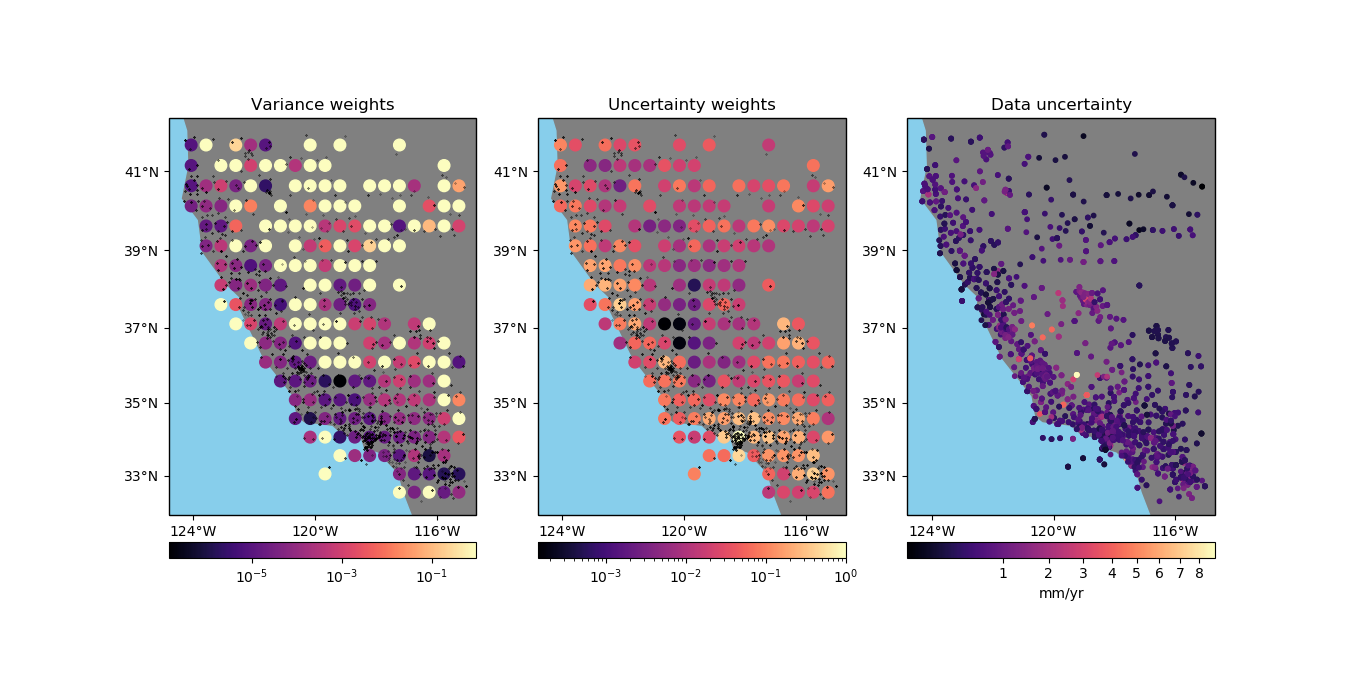
titles = ["Variance weights", "Uncertainty weights"]
weight_estimates = [variance_weights, uncertainty_weights]
for ax, title, w in zip(axes[:2], titles, weight_estimates):
ax.set_title(title)
# Plot the original data locations
ax.plot(*coordinates, ".k", transform=crs, markersize=0.5)
# Plot the weights using a logarithmic color scale to highlight the
# differences
pc = ax.scatter(
*block_coords, c=w, s=70, cmap="magma", transform=crs, norm=LogNorm()
)
plt.colorbar(pc, ax=ax, orientation="horizontal", pad=0.05)
vd.datasets.setup_california_gps_map(ax)
# Plot the original data uncertainties
ax = axes[2]
ax.set_title("Data uncertainty")
# Use a power law for the color scale because there is a lot of variability
# Convert m/year to mm/year to have smaller values on the color bar
pc = ax.scatter(
*coordinates,
c=data.std_up * 1000,
s=10,
transform=crs,
alpha=1,
cmap="magma",
norm=PowerNorm(gamma=1 / 2)
)
plt.colorbar(pc, ax=ax, orientation="horizontal", pad=0.05).set_label("mm/yr")
vd.datasets.setup_california_gps_map(ax)
plt.tight_layout()
plt.show()
Total running time of the script: ( 0 minutes 1.002 seconds)