Gridding with splines (cross-validated)

The verde.Spline has two main parameters that need to be configured:

1. mindist: the minimum distance between forces and data points

2. damping: the regularization parameter controlling smoothness

These parameters can be determined through cross-validation (see Model Selection) automatically using verde.SplineCV. It is very similar to verde.Spline but takes a set of parameter values instead of only one value. When calling verde.SplineCV.fit, the class will:

1. Create a spline for each combination of the input parameter sets

2. Calculate the cross-validation score for each spline using verde.cross_val_score

3. Pick the spline with the highest score

Out:

Score: 0.853

Best spline configuration:
  mindist: 50000.0
  damping: 0.001
/home/travis/build/fatiando/verde/examples/spline_cv.py:79: UserWarning: Tight layout not applied. The left and right margins cannot be made large enough to accommodate all axes decorations.
  plt.tight_layout()

import matplotlib.pyplot as plt
import cartopy.crs as ccrs
import pyproj
import numpy as np
import verde as vd

# We'll test this on the air temperature data from Texas
data = vd.datasets.fetch_texas_wind()
coordinates = (data.longitude.values, data.latitude.values)
region = vd.get_region(coordinates)

# Use a Mercator projection for our Cartesian gridder
projection = pyproj.Proj(proj="merc", lat_ts=data.latitude.mean())

# The output grid spacing will 15 arc-minutes
spacing = 15 / 60

# This spline will automatically perform cross-validation and search for the optimal
# parameter configuration.
spline = vd.SplineCV(dampings=(1e-5, 1e-3, 1e-1), mindists=(10e3, 50e3, 100e3))

# Fit the model on the data. Under the hood, the class will perform K-fold
# cross-validation for each the 3*3=9 parameter combinations and pick the one with the
# highest R² score.
spline.fit(projection(*coordinates), data.air_temperature_c)

# We can show the best R² score obtained in the cross-validation
print("\nScore: {:.3f}".format(spline.scores_.max()))

# And then the best spline parameters that produced this high score.
print("\nBest spline configuration:")
print("  mindist:", spline.mindist_)
print("  damping:", spline.damping_)

# Now we can create a geographic grid of air temperature by providing a projection
# function to the grid method and mask points that are too far from the observations
grid_full = spline.grid(
    region=region,
    spacing=spacing,
    projection=projection,
    dims=["latitude", "longitude"],
    data_names=["temperature"],
)
grid = vd.distance_mask(
    coordinates, maxdist=3 * spacing * 111e3, grid=grid_full, projection=projection
)

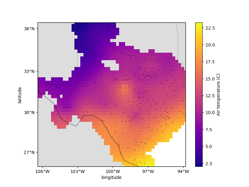
# Plot the grid and the original data points
plt.figure(figsize=(8, 6))
ax = plt.axes(projection=ccrs.Mercator())
ax.set_title("Air temperature gridded with biharmonic spline")
ax.plot(*coordinates, ".k", markersize=1, transform=ccrs.PlateCarree())
tmp = grid.temperature.plot.pcolormesh(
    ax=ax, cmap="plasma", transform=ccrs.PlateCarree(), add_colorbar=False
)
plt.colorbar(tmp).set_label("Air temperature (C)")
# Use an utility function to add tick labels and land and ocean features to the map.
vd.datasets.setup_texas_wind_map(ax, region=region)
plt.tight_layout()
plt.show()