Note
Click here to download the full example code
Model Selection
In Evaluating Performance, we saw how to check the performance of an interpolator using
cross-validation. We found that the default parameters for verde.Spline are not
good for predicting our sample air temperature data. Now, let’s see how we can tune the
Spline to improve the cross-validation performance.
Once again, we’ll start by importing the required packages and loading our sample data.
import numpy as np
import matplotlib.pyplot as plt
import cartopy.crs as ccrs
import itertools
import pyproj
import verde as vd

data = vd.datasets.fetch_texas_wind()

# Use Mercator projection because Spline is a Cartesian gridder
projection = pyproj.Proj(proj="merc", lat_ts=data.latitude.mean())
proj_coords = projection(data.longitude.values, data.latitude.values)

region = vd.get_region((data.longitude, data.latitude))
# The desired grid spacing in degrees (converted to meters using 1 degree approx. 111km)
spacing = 15 / 60
Before we begin tuning, let’s reiterate what the results were with the default parameters.
spline_default = vd.Spline()
score_default = np.mean(
    vd.cross_val_score(spline_default, proj_coords, data.air_temperature_c)
)
spline_default.fit(proj_coords, data.air_temperature_c)
print("R² with defaults:", score_default)
Out:
R² with defaults: 0.7960368854849694
Tuning
Spline has many parameters that can be set to modify the final result.
Mainly the damping regularization parameter and the mindist “fudge factor”
which smooths the solution. Would changing the default values give us a better score?
We can answer these questions by changing the values in our spline and
re-evaluating the model score repeatedly for different values of these parameters.
Let’s test the following combinations:
dampings = [None, 1e-4, 1e-3, 1e-2]
mindists = [5e3, 10e3, 50e3, 100e3]

# Use itertools to create a list with all combinations of parameters to test
parameter_sets = [
    dict(damping=combo[0], mindist=combo[1])
    for combo in itertools.product(dampings, mindists)
]
print("Number of combinations:", len(parameter_sets))
print("Combinations:", parameter_sets)
Out:
Number of combinations: 16
Combinations: [{'damping': None, 'mindist': 5000.0}, {'damping': None, 'mindist': 10000.0}, {'damping': None, 'mindist': 50000.0}, {'damping': None, 'mindist': 100000.0}, {'damping': 0.0001, 'mindist': 5000.0}, {'damping': 0.0001, 'mindist': 10000.0}, {'damping': 0.0001, 'mindist': 50000.0}, {'damping': 0.0001, 'mindist': 100000.0}, {'damping': 0.001, 'mindist': 5000.0}, {'damping': 0.001, 'mindist': 10000.0}, {'damping': 0.001, 'mindist': 50000.0}, {'damping': 0.001, 'mindist': 100000.0}, {'damping': 0.01, 'mindist': 5000.0}, {'damping': 0.01, 'mindist': 10000.0}, {'damping': 0.01, 'mindist': 50000.0}, {'damping': 0.01, 'mindist': 100000.0}]
Now we can loop over the combinations and collect the scores for each parameter set.
spline = vd.Spline()
scores = []
for params in parameter_sets:
    spline.set_params(**params)
    score = np.mean(vd.cross_val_score(spline, proj_coords, data.air_temperature_c))
    scores.append(score)
print(scores)
Out:
[-6.672752084450996, 0.4845403172681578, 0.8383522700290031, 0.8371988991060888, 0.8351153077295754, 0.8316607509400296, 0.849262993117369, 0.8418400888505818, 0.8371795091862098, 0.8412200336661682, 0.8529555082414106, 0.8521727667594355, 0.8401945161937409, 0.8330182923876521, 0.8441706458561657, 0.849114559135252]
The largest score will yield the best parameter combination.
best = np.argmax(scores)
print("Best score:", scores[best])
print("Score with defaults:", score_default)
print("Best parameters:", parameter_sets[best])
Out:
Best score: 0.8529555082414106
Score with defaults: 0.7960368854849694
Best parameters: {'damping': 0.001, 'mindist': 50000.0}
That is a nice improvement over our previous score!
This type of tuning is important and should always be performed when using a new gridder or a new dataset. However, the above implementation requires a lot of coding. Fortunately, Verde provides convenience classes that perform the cross-validation and tuning automatically when fitting a dataset.
Cross-validated gridders
The verde.SplineCV class provides a cross-validated version of
verde.Spline. It has almost the same interface but does all of the above
automatically when fitting a dataset. The only difference is that you must provide a
list of damping and mindist parameters to try instead of only a single value:
Calling fit will run a grid search over all parameter
combinations to find the one that maximizes the cross-validation score.
spline.fit(proj_coords, data.air_temperature_c)
Out:
SplineCV(client=None, cv=None, dampings=[None, 0.0001, 0.001, 0.01],
         delayed=False, engine='auto', force_coords=None,
         mindists=[5000.0, 10000.0, 50000.0, 100000.0])
The estimated best damping and mindist, as well as the cross-validation scores, are stored in class attributes:
Out:
Highest score: 0.8529555082414106
Best damping: 0.001
Best mindist: 50000.0
The cross-validated gridder can be used like any other gridder (including in
verde.Chain and verde.Vector):
Out:
<xarray.Dataset>
Dimensions:      (latitude: 43, longitude: 51)
Coordinates:
  * longitude    (longitude) float64 -106.4 -106.1 -105.9 ... -94.06 -93.8
  * latitude     (latitude) float64 25.91 26.16 26.41 ... 35.91 36.16 36.41
Data variables:
    temperature  (latitude, longitude) float64 19.42 19.42 19.43 ... 7.536 7.765
Attributes:
    metadata:  Generated by SplineCV(client=None, cv=None, dampings=[None, 0....
Like verde.cross_val_score, SplineCV can also run the
grid search in parallel using Dask by specifying the
delayed attribute:
Unlike verde.cross_val_score, calling fit
does not result in dask.delayed objects. The full grid search is
executed and the optimal parameters are found immediately.
spline.fit(proj_coords, data.air_temperature_c)

print("Best damping:", spline.damping_)
print("Best mindist:", spline.mindist_)
Out:
Best damping: 0.001
Best mindist: 50000.0
The one caveat is the that the scores_ attribute will be a list of
dask.delayed objects instead because the scores are only computed as
intermediate values in the scheduled computations.
print("Delayed scores:", spline.scores_)
Out:
Delayed scores: [Delayed('mean-79241980-a294-4d3b-a8c4-de0e0a977dac'), Delayed('mean-4f644052-6482-4276-a878-cf97f2cbdddd'), Delayed('mean-ca309ce2-5599-4f23-81ac-12029c87c9e4'), Delayed('mean-3e82f14c-9ec2-4cd3-b671-b31fb80ae056'), Delayed('mean-6f07a2ee-a972-4776-ae6e-8d3da7b549d1'), Delayed('mean-25c53a9f-a563-478d-b2bb-55763dfa6024'), Delayed('mean-1e4e1bac-05cf-4e0f-b0a1-87fb6ec92e0b'), Delayed('mean-5a5e4b0d-2480-4bc5-a018-fb5532d3ff21'), Delayed('mean-70b1a4f1-32ce-4abc-8394-9bd5981ea463'), Delayed('mean-e209b8f5-6738-499d-a9de-4fa0c1417162'), Delayed('mean-693b0351-e407-45cb-a80d-7c414a9cb1df'), Delayed('mean-4f8c2d4c-887e-4c26-bc16-8d397cd4e26d'), Delayed('mean-67467046-3878-40dd-9e21-17b052d40447'), Delayed('mean-a8b4e183-04ad-4440-8e71-422684e645ab'), Delayed('mean-ee21a1a0-c205-41c0-99f9-c1c7fb06a4b8'), Delayed('mean-6204781c-5f80-46b2-b6f6-21e927cccee9')]
Calling dask.compute on the scores will calculate their values but
will unfortunately run the entire grid search again. So using
delayed=True is not recommended if you need the scores of each parameter
combination.
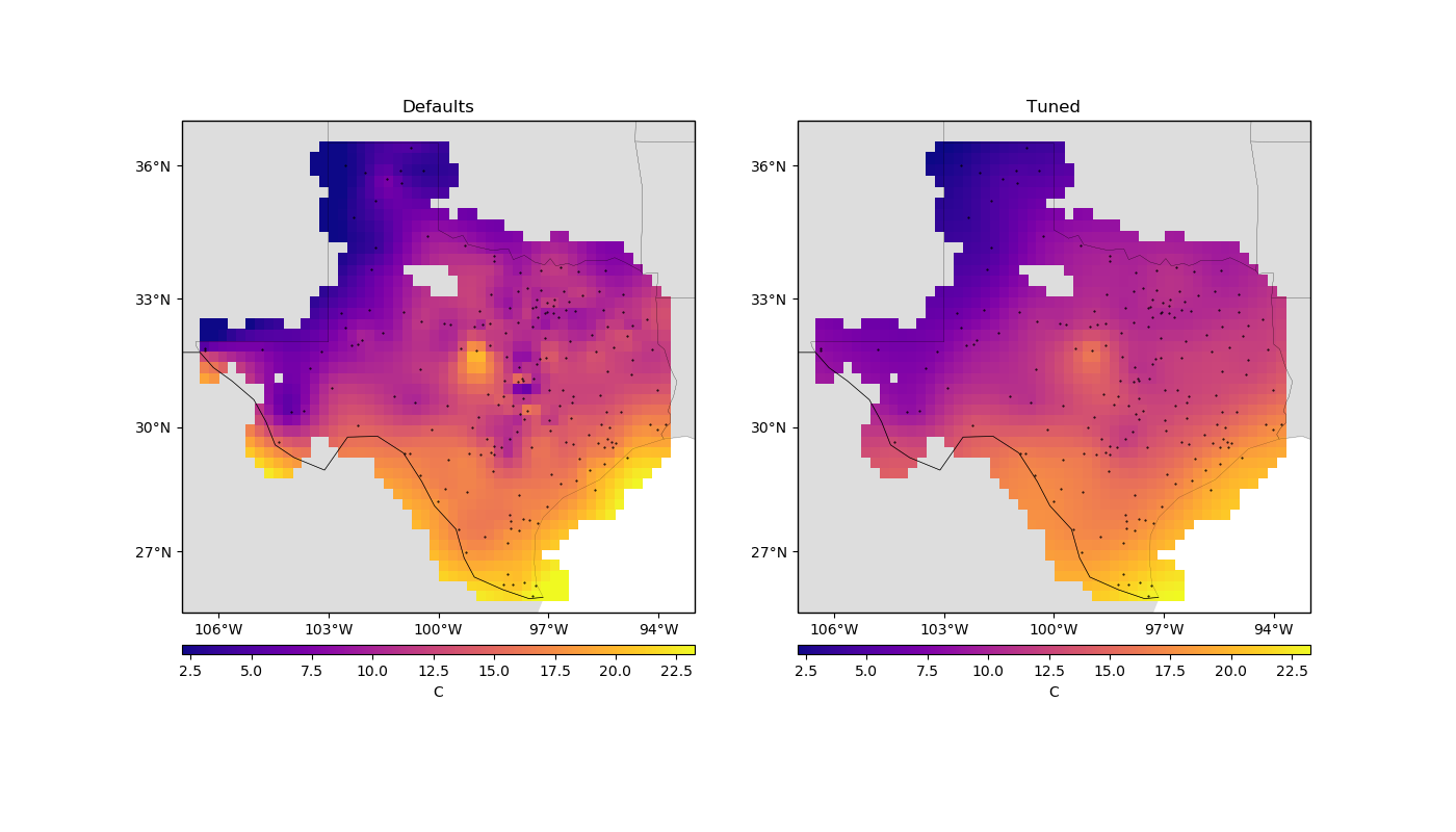
The importance of tuning
To see the difference that tuning has on the results, we can make a grid with the best configuration and see how it compares to the default result.
grid_default = spline_default.grid(
    region=region,
    spacing=spacing,
    projection=projection,
    dims=["latitude", "longitude"],
    data_names=["temperature"],
)
Let’s plot our grids side-by-side:
mask = vd.distance_mask(
    (data.longitude, data.latitude),
    maxdist=3 * spacing * 111e3,
    coordinates=vd.grid_coordinates(region, spacing=spacing),
    projection=projection,
)

grid = grid.where(mask)
grid_default = grid_default.where(mask)

plt.figure(figsize=(14, 8))
for i, title, grd in zip(range(2), ["Defaults", "Tuned"], [grid_default, grid]):
    ax = plt.subplot(1, 2, i + 1, projection=ccrs.Mercator())
    ax.set_title(title)
    pc = grd.temperature.plot.pcolormesh(
        ax=ax,
        cmap="plasma",
        transform=ccrs.PlateCarree(),
        vmin=data.air_temperature_c.min(),
        vmax=data.air_temperature_c.max(),
        add_colorbar=False,
        add_labels=False,
    )
    plt.colorbar(pc, orientation="horizontal", aspect=50, pad=0.05).set_label("C")
    ax.plot(
        data.longitude, data.latitude, ".k", markersize=1, transform=ccrs.PlateCarree()
    )
    vd.datasets.setup_texas_wind_map(ax)
plt.tight_layout()
plt.show()
Out:
/home/travis/build/fatiando/verde/tutorials/model_selection.py:208: UserWarning: Tight layout not applied. The left and right margins cannot be made large enough to accommodate all axes decorations.
  plt.tight_layout()
Notice that, for sparse data like these, smoother models tend to be better predictors. This is a sign that you should probably not trust many of the short wavelength features that we get from the defaults.
Total running time of the script: ( 0 minutes 2.678 seconds)