4. Random coordinates#
Sometimes, we need to generate a random spread of points in 1 or more
dimensions. This can be used for random sampling methods or simply to
generate some synthetic data on which to test new methods. Generating
uniformly distributed values using numpy.random is great but doing
so in more than 1 dimension involves some boilerplate code that could be
automated. Bordado offers functions random_coordinates and
random_coordinates_spherical for this purpose. This is how they
work.
import bordado as bd
import matplotlib.pyplot as plt
import pygmt
4.1. Generating random points#
To generate uniformly distributed random 2D point coordinates, we use bordado.random_coordinates like so:
region = (0, 20, -45, -30)
coordinates = bd.random_coordinates(region, size=50)

for i, c in enumerate(coordinates):
    print(f"coordinate {i}:\n{c}\n")
coordinate 0:
[15.52784602  6.39780646 13.07887575 19.16855283  6.04481505  9.03574181
 12.60014114  8.15085158  6.10755689  8.85007442 12.80343388 13.38048145
 17.37596646  9.24343149 13.84581915 16.87805113  2.31944968 17.99277566
  4.22725465  2.96614266 16.13429178 18.1040038  13.76914217 16.38549962
  1.41518575  6.8663168  11.21824917  8.83161776 15.37812111 16.44122641
 12.33845814  9.01505108  2.73939222  2.49927411 19.82415786  8.39089365
  0.1750859  13.31634254  8.76757003  0.86587759 10.10106497  1.64487265
  0.36911055  4.1058305  14.4610567   9.10998553  6.3244591  13.9123466
 12.25203381  5.07900578]

coordinate 1:
[-43.39062161 -34.89581084 -40.97528541 -34.71366905 -44.88600536
 -40.08063149 -37.59718258 -40.58848351 -38.88070512 -41.47423151
 -38.27730982 -33.43264527 -41.23339859 -37.99157852 -37.45438641
 -39.3338382  -34.0446157  -39.05981696 -43.80800703 -38.96390674
 -36.57850193 -40.12392515 -38.64029873 -42.52158388 -40.03147855
 -35.80362144 -42.46939855 -36.06872896 -30.13124192 -36.2530416
 -44.40541845 -40.87392707 -39.04887015 -32.12328814 -34.08891496
 -42.72632816 -41.00433603 -43.61598859 -44.21582561 -34.17153746
 -39.61362259 -40.33242764 -43.7608447  -37.28291664 -39.51370868
 -39.92677845 -37.74346183 -34.84429854 -30.14443363 -38.4941258 ]
Since the region has 4 elements, it is assumed that there are two dimensions
in our problem and so 2 coordinates arrays are generated. Because the points are
uniformly distributed, there is only a size argument and no spacing like in
bordado.grid_coordinates or bordado.line_coordinates.
Hint
The values above will be different every time we run the function because
it will instantiate a new numpy.random.default_rng every time. We
can control the randomness by passing a random_seed argument. This can
be an integer seed or a numpy.random.Generator.
Let’s plot these points to see their distribution:
fig, ax = plt.subplots(1, 1, figsize=(8, 6), layout="constrained")
ax.plot(*coordinates, "o")
ax.set_aspect("equal")
ax.set_xlim(*region[:2])
ax.set_ylim(*region[2:])
ax.set_xlabel("Easting")
ax.set_ylabel("Northing")
ax.grid()
plt.show()
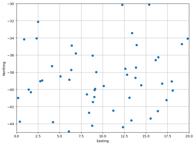
As expected, they are random and with no bias inside the given region (hence, uniformly distributed).
4.2. Random points on the sphere#
The method above is useful, but it shouldn’t be used with geographic longitude and latitude coordinates. Let’s illustrate why with an example. We’ll generate random points distributed globally:
region = (0, 360, -90, 90)  # W, E, S, N in degrees
size = 3000

coordinates = bd.random_coordinates(region, size)

fig, ax = plt.subplots(1, 1, figsize=(8, 6), layout="constrained")
ax.plot(*coordinates, ".")
ax.set_aspect("equal")
ax.set_xlim(*region[:2])
ax.set_ylim(*region[2:])
ax.set_xlabel("Longitude")
ax.set_ylabel("Latitude")
ax.grid()
plt.show()
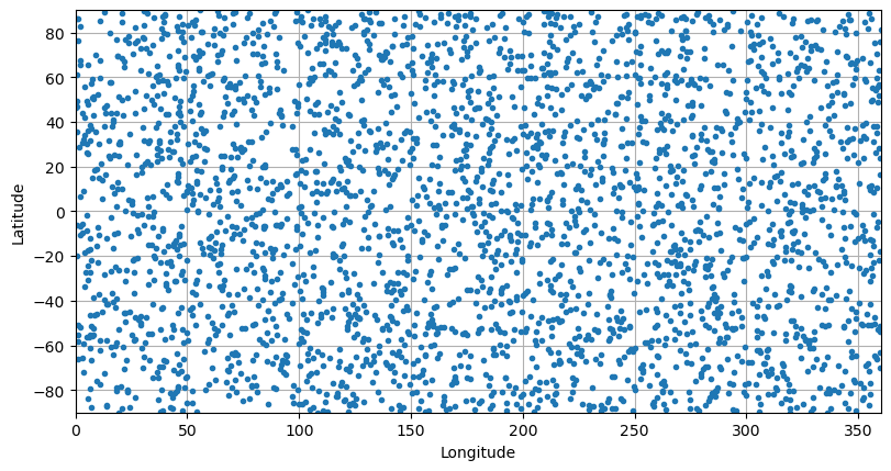
Plotted like this, things seem fine. But this type of plot can be very misleading for geographic data. If I plot them on a map using a cartographic projection, a pattern will appear:
fig = pygmt.Figure()
fig.coast(land="#cccccc", region="g", projection="W20c", frame="afg")
fig.plot(x=coordinates[0], y=coordinates[1], style="c0.1c", fill="seagreen")
fig.show()
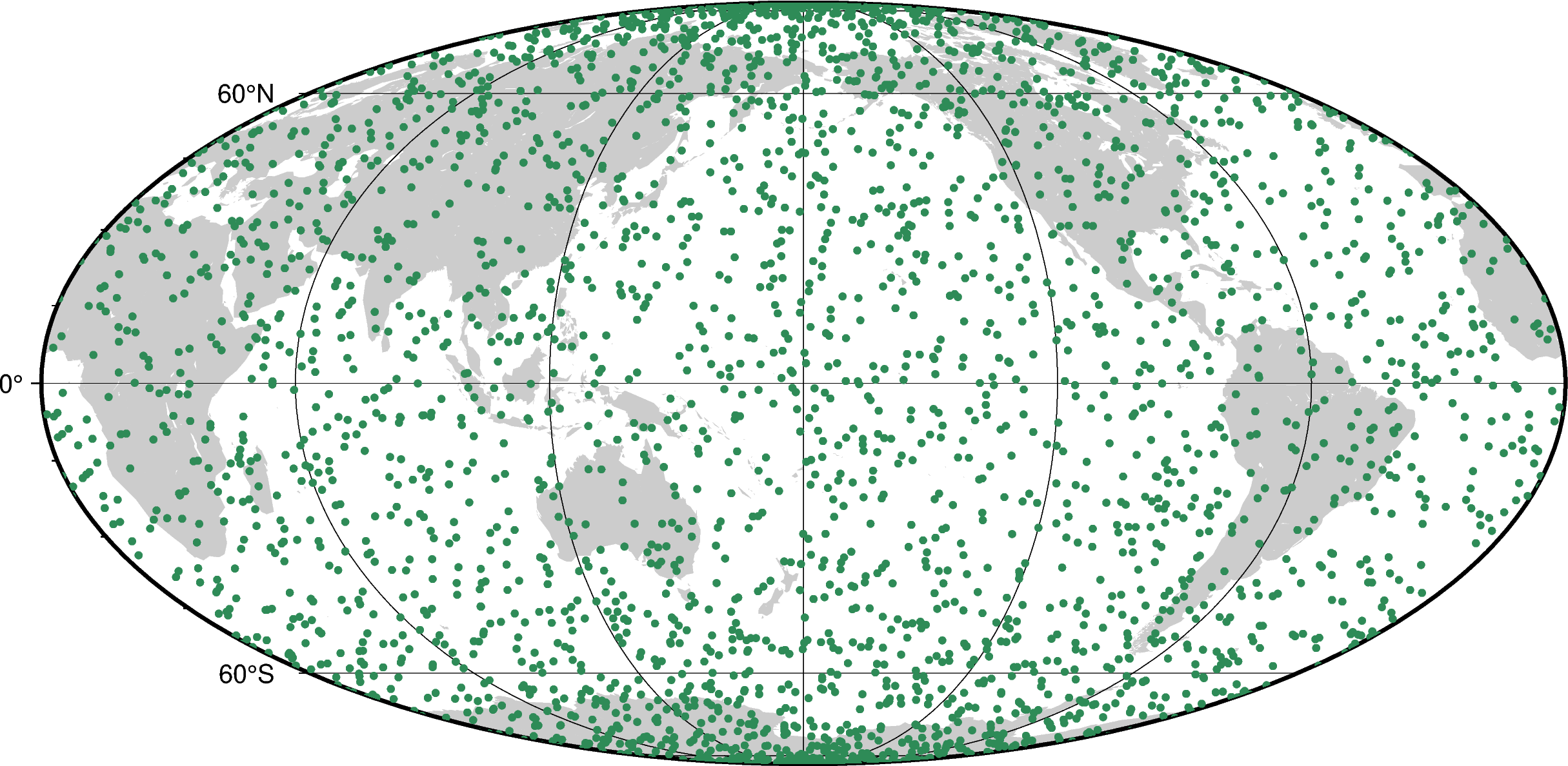
Now we can see that the concentration of points is larger at the poles than at the equator. This is because the meridians of longitude converge at the poles. Hence, a degree of longitude corresponds to a smaller and smaller physical size on the surface of the Earth towards the poles.
See also
The map above was generated with a Mollweide projection, which is an equal-area projection.
To generate random points on a sphere that have a uniform distribution, we
can use bordado.random_coordinates_spherical, which accounts for this
convergence of meridians:
coordinates_sphere = bd.random_coordinates_spherical(region, size)

fig = pygmt.Figure()
fig.coast(land="#cccccc", region="g", projection="W20c", frame="afg")
fig.plot(x=coordinates_sphere[0], y=coordinates_sphere[1], style="c0.1c", fill="seagreen")
fig.show()
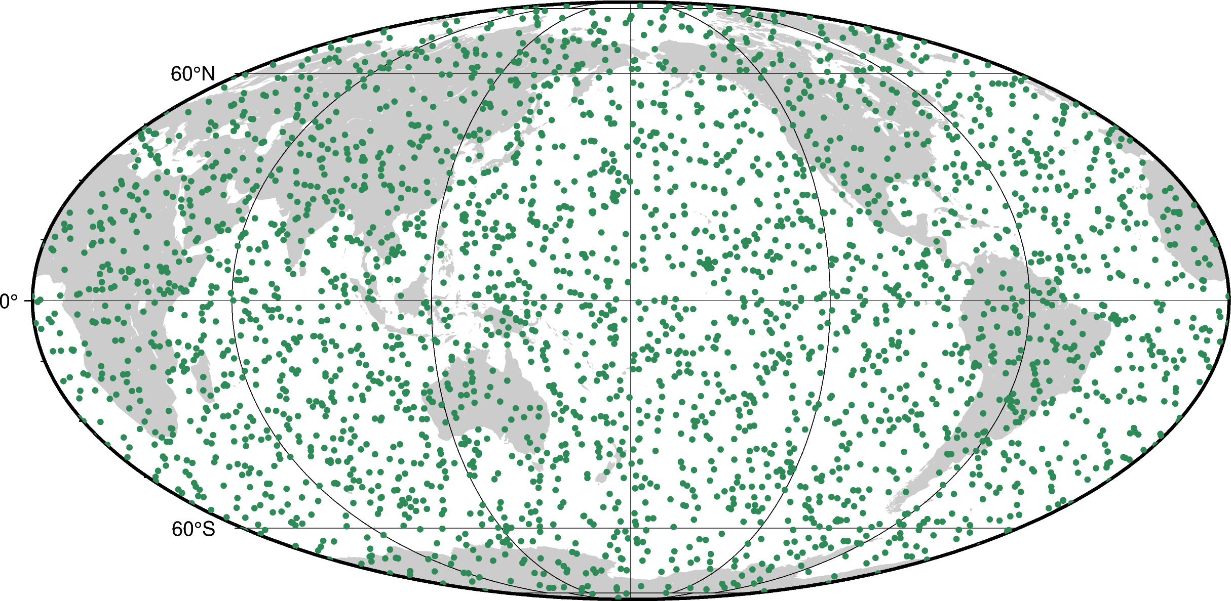
Notice that now the point concentration is uniform on the Earth.
4.3. What’s next#
Now that we can make some synthetic data with random points, let’s see how we can split and segment the data based on spatial blocks and windows in “Splitting points into blocks”.
Have questions?
Please ask on any of the Fatiando a Terra community channels!