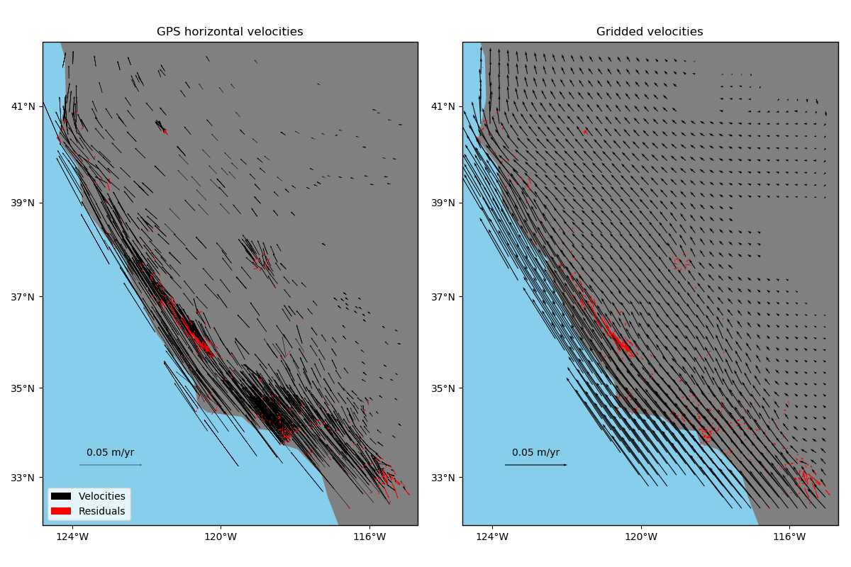
Gridding 2D vectors (coupled)

One way of gridding vector data would be grid each component separately using verde.Spline and verde.Vector. Alternatively, verde.VectorSpline2D can grid two components simultaneously in a way that couples them through elastic deformation theory. This is particularly suited, though not exclusive, to data that represent elastic/semi-elastic deformation, like horizontal GPS velocities.

Out:

Cross-validation R^2 score: 0.97

import matplotlib.pyplot as plt
import cartopy.crs as ccrs
import numpy as np
import pyproj
import verde as vd


# Fetch the GPS data from the U.S. West coast. We'll grid only the horizontal components
# of the velocities
data = vd.datasets.fetch_california_gps()
coordinates = (data.longitude.values, data.latitude.values)
region = vd.get_region(coordinates)
# Use a Mercator projection because VectorSpline2D is a Cartesian gridder
projection = pyproj.Proj(proj="merc", lat_ts=data.latitude.mean())

# Split the data into a training and testing set. We'll fit the gridder on the training
# set and use the testing set to evaluate how well the gridder is performing.
train, test = vd.train_test_split(
    projection(*coordinates), (data.velocity_east, data.velocity_north), random_state=0
)

# We'll make a 15 arc-minute grid in the end.
spacing = 15 / 60

# Chain together a blocked mean to avoid aliasing, a polynomial trend to take care of
# the increase toward the coast, and finally the vector gridder using Poisson's ratio
# 0.5 to couple the two horizontal components.
chain = vd.Chain(
    [
        ("mean", vd.BlockReduce(np.mean, spacing * 111e3)),
        ("trend", vd.Vector([vd.Trend(degree=1) for i in range(2)])),
        ("spline", vd.VectorSpline2D(poisson=0.5, mindist=10e3)),
    ]
)
# Fit on the training data
chain.fit(*train)
# And score on the testing data. The best possible score is 1, meaning a perfect
# prediction of the test data.
score = chain.score(*test)
print("Cross-validation R^2 score: {:.2f}".format(score))

# Interpolate our horizontal GPS velocities onto a regular geographic grid and mask the
# data that are far from the observation points
grid_full = chain.grid(
    region, spacing=spacing, projection=projection, dims=["latitude", "longitude"]
)
grid = vd.distance_mask(
    (data.longitude, data.latitude),
    maxdist=2 * spacing * 111e3,
    grid=grid_full,
    projection=projection,
)

# Calculate residuals between the predictions and the original input data. Even though
# we aren't using regularization or regularly distributed forces, the prediction won't
# be perfect because of the BlockReduce operation. We fit the gridder on the reduced
# observations, not the original data.
predicted = chain.predict(projection(*coordinates))
residuals = (data.velocity_east - predicted[0], data.velocity_north - predicted[1])

# Make maps of the original velocities, the gridded velocities, and the residuals
fig, axes = plt.subplots(
    1, 2, figsize=(12, 8), subplot_kw=dict(projection=ccrs.Mercator())
)
crs = ccrs.PlateCarree()
# Plot the observed data and the residuals
ax = axes[0]
tmp = ax.quiver(
    data.longitude.values,
    data.latitude.values,
    data.velocity_east.values,
    data.velocity_north.values,
    scale=0.3,
    transform=crs,
    width=0.001,
    label="Velocities",
)
ax.quiverkey(tmp, 0.13, 0.18, 0.05, label="0.05 m/yr", coordinates="figure")
ax.quiver(
    data.longitude.values,
    data.latitude.values,
    residuals[0].values,
    residuals[1].values,
    scale=0.3,
    transform=crs,
    color="r",
    width=0.001,
    label="Residuals",
)
ax.set_title("GPS horizontal velocities")
ax.legend(loc="lower left")
vd.datasets.setup_california_gps_map(ax)
# Plot the gridded data and the residuals
ax = axes[1]
tmp = ax.quiver(
    grid.longitude.values,
    grid.latitude.values,
    grid.east_component.values,
    grid.north_component.values,
    scale=0.3,
    transform=crs,
    width=0.002,
)
ax.quiverkey(tmp, 0.63, 0.18, 0.05, label="0.05 m/yr", coordinates="figure")
ax.quiver(
    data.longitude.values,
    data.latitude.values,
    residuals[0].values,
    residuals[1].values,
    scale=0.3,
    transform=crs,
    color="r",
    width=0.001,
)
ax.set_title("Gridded velocities")
vd.datasets.setup_california_gps_map(ax)
plt.tight_layout()
plt.show()

Total running time of the script: ( 0 minutes 2.849 seconds)