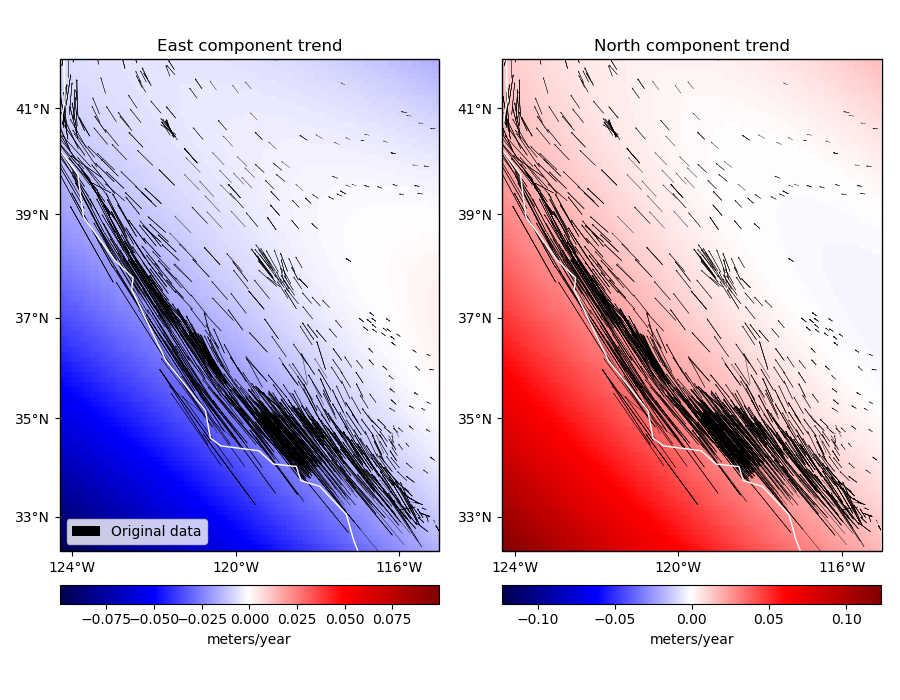
Trends in vector data

Verde provides the verde.Trend class to estimate a polynomial trend and the verde.Vector class to apply any combination of estimators to each component of vector data, like GPS velocities. You can access each component as a separate (fitted) verde.Trend instance or operate on all vector components directly using using verde.Vector.predict, verde.Vector.grid, etc, or chaining it with a vector interpolator using verde.Chain.

Out:

Vector trend estimator: Vector(components=[Trend(degree=2), Trend(degree=2)])
East component trend: Trend(degree=2)
East trend coefficients: [-2.63027348e+01  1.65325273e-01  3.15539485e-01 -2.54890059e-04
 -1.04529316e-03 -8.02571744e-04]
North component trend: Trend(degree=2)
North trend coefficients: [ 4.41288370e+01 -3.04681356e-01 -3.63276562e-01  5.27969954e-04
  1.22423033e-03  8.52765037e-04]

Gridded 2-component trend:
<xarray.Dataset>
Dimensions:          (latitude: 97, longitude: 94)
Coordinates:
  * longitude        (longitude) float64 235.7 235.8 235.9 ... 244.8 244.9 245.0
  * latitude         (latitude) float64 32.29 32.39 32.49 ... 41.7 41.8 41.9
Data variables:
    east_component   (latitude, longitude) float64 -0.09947 ... -0.01609
    north_component  (latitude, longitude) float64 0.1229 0.1213 ... 0.01632
Attributes:
    metadata:  Generated by Vector(components=[Trend(degree=2), Trend(degree=...

import matplotlib.pyplot as plt
import cartopy.crs as ccrs
import numpy as np
import verde as vd


# Fetch the GPS data from the U.S. West coast. The data has a strong trend toward the
# North-West because of the relative movement along the San Andreas Fault System.
data = vd.datasets.fetch_california_gps()

# We'll fit a degree 2 trend on both the East and North components and weight the data
# using the inverse of the variance of each component.
# Note: Never use [Trend(...)]*2 as an argument to Vector. This creates references
# to the same Trend instance and will mess up the fitting.
trend = vd.Vector([vd.Trend(degree=2) for i in range(2)])
weights = vd.variance_to_weights((data.std_east ** 2, data.std_north ** 2))
trend.fit(
    coordinates=(data.longitude, data.latitude),
    data=(data.velocity_east, data.velocity_north),
    weights=weights,
)
print("Vector trend estimator:", trend)

# The separate Trend objects for each component can be accessed through the 'components'
# attribute. You could grid them individually if you wanted.
print("East component trend:", trend.components[0])
print("East trend coefficients:", trend.components[0].coef_)
print("North component trend:", trend.components[1])
print("North trend coefficients:", trend.components[1].coef_)

# We can make a grid with both trend components as data variables
grid = trend.grid(spacing=0.1, dims=["latitude", "longitude"])
print("\nGridded 2-component trend:")
print(grid)


# Now we can map both trends along with the original data for comparison
fig, axes = plt.subplots(
    1, 2, figsize=(9, 7), subplot_kw=dict(projection=ccrs.Mercator())
)
crs = ccrs.PlateCarree()
# Plot the two trend components
titles = ["East component trend", "North component trend"]
components = [grid.east_component, grid.north_component]
for ax, component, title in zip(axes, components, titles):
    ax.set_title(title)
    # Plot the trend in pseudo color
    maxabs = vd.maxabs(component)
    tmp = component.plot.pcolormesh(
        ax=ax,
        vmin=-maxabs,
        vmax=maxabs,
        cmap="seismic",
        transform=crs,
        add_colorbar=False,
        add_labels=False,
    )
    cb = plt.colorbar(tmp, ax=ax, orientation="horizontal", pad=0.05)
    cb.set_label("meters/year")
    # Plot the original data
    ax.quiver(
        data.longitude.values,
        data.latitude.values,
        data.velocity_east.values,
        data.velocity_north.values,
        scale=0.2,
        transform=crs,
        color="k",
        width=0.001,
        label="Original data",
    )
    # Setup the map ticks
    vd.datasets.setup_california_gps_map(
        ax, land=None, ocean=None, region=vd.get_region((data.longitude, data.latitude))
    )
    ax.coastlines(color="white")
axes[0].legend(loc="lower left")
plt.tight_layout()
plt.show()

Total running time of the script: ( 0 minutes 0.231 seconds)