Note
Click here to download the full example code
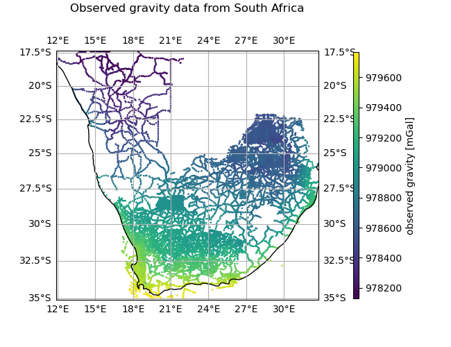
Land Gravity Data from South Africa
Land gravity survey performed in January 1986 within the boundaries of the
Republic of South Africa. The data was made available by the National Centers
for Environmental Information (NCEI) (formerly
NGDC) and are in the public domain. The
entire dataset is stored in a pandas.DataFrame with columns:
longitude, latitude, elevation (above sea level) and gravity(mGal). See the
documentation for harmonica.datasets.fetch_south_africa_gravity for
more information.
Out:
       latitude  longitude  elevation    gravity
0     -34.39150   17.71900     -589.0  979724.79
1     -34.48000   17.76100     -495.0  979712.90
2     -34.35400   17.77433     -406.0  979725.89
3     -34.13900   17.78500     -267.0  979701.20
4     -34.42200   17.80500     -373.0  979719.00
...         ...        ...        ...        ...
14554 -17.95833   21.22500     1053.1  978182.09
14555 -17.98333   21.27500     1033.3  978183.09
14556 -17.99166   21.70833     1041.8  978182.69
14557 -17.95833   21.85000     1033.3  978193.18
14558 -17.94166   21.98333     1022.6  978211.38

[14559 rows x 4 columns]
import matplotlib.pyplot as plt
import cartopy.crs as ccrs
import verde as vd
import harmonica as hm

# Fetch the data in a pandas.DataFrame
data = hm.datasets.fetch_south_africa_gravity()
print(data)

# Plot the observations in a Mercator map using Cartopy
fig = plt.figure(figsize=(6.5, 5))
ax = plt.axes(projection=ccrs.Mercator())
ax.set_title("Observed gravity data from South Africa", pad=25)
tmp = ax.scatter(
    data.longitude,
    data.latitude,
    c=data.gravity,
    s=0.8,
    cmap="viridis",
    transform=ccrs.PlateCarree(),
)
plt.colorbar(
    tmp, ax=ax, label="observed gravity [mGal]", aspect=50, pad=0.1, shrink=0.92
)
ax.set_extent(vd.get_region((data.longitude, data.latitude)))
ax.gridlines(draw_labels=True)
ax.coastlines()
plt.show()
Total running time of the script: ( 0 minutes 0.959 seconds)