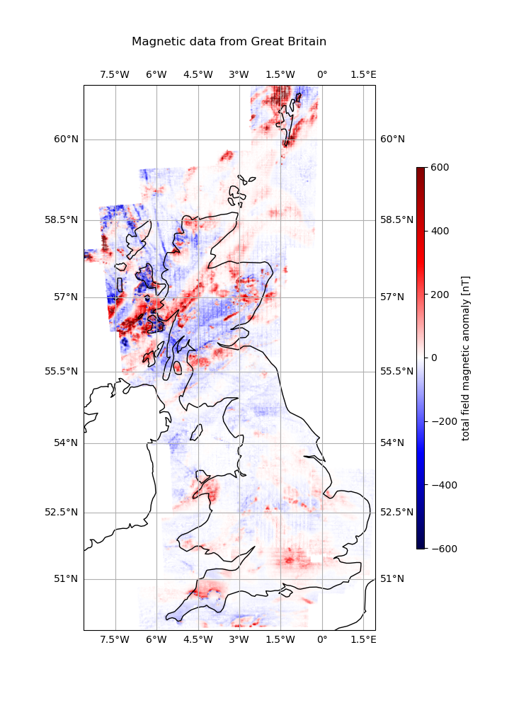
Total Field Magnetic Anomaly from Great Britain¶

These data are a complete airborne survey of the entire Great Britain conducted between 1955 and 1965. The data are made available by the British Geological Survey (BGS) through their geophysical data portal.

License: Open Government License

The columns of the data table are longitude, latitude, total-field magnetic anomaly (nanoTesla), observation height relative to the WGS84 datum (in meters), survey area, and line number and line segment for each data point.

Latitude, longitude, and elevation data converted from original OSGB36 (epsg:27700) coordinate system to WGS84 (epsg:4326) using to_crs function in GeoPandas.

See the original data for more processing information.

If the file isn’t already in your data directory, it will be downloaded automatically.

Out:

       survey_area line-number-segment  ...  altitude_m  total_field_anomaly_nt
0       CA55_NORTH               FL1-1  ...       842.0                      62
1       CA55_NORTH               FL1-1  ...       713.0                      56
2       CA55_NORTH               FL1-1  ...       364.0                      30
3       CA55_NORTH               FL1-1  ...       364.0                      31
4       CA55_NORTH               FL1-1  ...       370.0                      44
...            ...                 ...  ...         ...                     ...
541503        HG65     FL-3(TL10-24)-1  ...      1084.0                      64
541504        HG65     FL-3(TL10-24)-1  ...      1098.0                      74
541505        HG65     FL-3(TL10-24)-1  ...      1088.0                      94
541506        HG65     FL-3(TL10-24)-1  ...      1077.0                     114
541507        HG65     FL-3(TL10-24)-1  ...      1064.0                     120

[541508 rows x 6 columns]

import matplotlib.pyplot as plt
import cartopy.crs as ccrs
import verde as vd
import harmonica as hm
import numpy as np

# Fetch the data in a pandas.DataFrame
data = hm.datasets.fetch_britain_magnetic()
print(data)

# Plot the observations in a Mercator map using Cartopy
fig = plt.figure(figsize=(7.5, 10))
ax = plt.axes(projection=ccrs.Mercator())
ax.set_title("Magnetic data from Great Britain", pad=25)
maxabs = np.percentile(data.total_field_anomaly_nt, 99)
tmp = ax.scatter(
    data.longitude,
    data.latitude,
    c=data.total_field_anomaly_nt,
    s=0.001,
    cmap="seismic",
    vmin=-maxabs,
    vmax=maxabs,
    transform=ccrs.PlateCarree(),
)
plt.colorbar(
    tmp,
    ax=ax,
    label="total field magnetic anomaly [nT]",
    orientation="vertical",
    aspect=50,
    shrink=0.7,
    pad=0.1,
)
ax.set_extent(vd.get_region((data.longitude, data.latitude)))
ax.gridlines(draw_labels=True)
ax.coastlines(resolution="50m")
plt.show()

Total running time of the script: ( 0 minutes 7.648 seconds)

Gallery generated by Sphinx-Gallery

Harmonica v0.3.3

Total Field Magnetic Anomaly from Great Britain¶