Magnetic airborne survey of Britain
Note
Click here to download the full example code
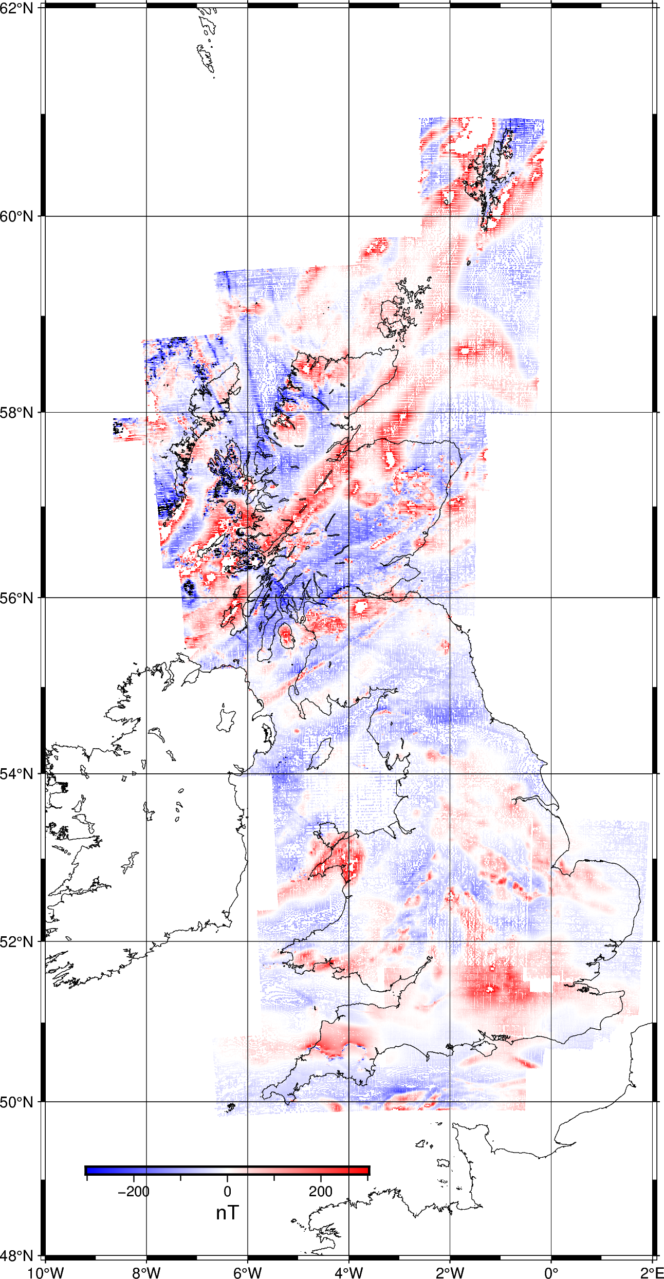
Magnetic airborne survey of Britain
This is a digitization of an airborne magnetic survey of Britain. Data are sampled where flight lines crossed contours on the archive maps. Contains only the total field magnetic anomaly, not the magnetic field intensity measurements or corrections.
Unfortunately, the exact date of measurements is not available (only the year).
Contains British Geological Survey materials © UKRI 2021.
Original source: British Geological Survey
import numpy as np
import pandas as pd
import pygmt

import ensaio
Download and cache the data and return the path to it on disk
fname = ensaio.fetch_britain_magnetic(version=1)
print(fname)
Out:
/home/runner/work/_temp/cache/ensaio/v1/britain-magnetic.csv.xz
Load the CSV formatted data with pandas
data = pd.read_csv(fname)
data
Make a PyGMT map with the data points colored by the total field magnetic anomaly.
fig = pygmt.Figure()
scale = np.percentile(data.total_field_anomaly_nt, 95)
pygmt.makecpt(cmap="polar", series=[-scale, scale])
fig.plot(
    x=data.longitude,
    y=data.latitude,
    style="c0.02c",
    color=data.total_field_anomaly_nt,
    cmap=True,
    projection="M15c",
)
fig.colorbar(frame='af+l"nT"', position="jBL+h+w7c/0.2c+o1/2")
fig.coast(shorelines=True)
fig.basemap(frame="afg")
fig.show()
Out:
<IPython.core.display.Image object>
Total running time of the script: ( 0 minutes 21.924 seconds)