GPS velocities (3-component) for the Alps
Note
Click here to download the full example code
GPS velocities (3-component) for the Alps
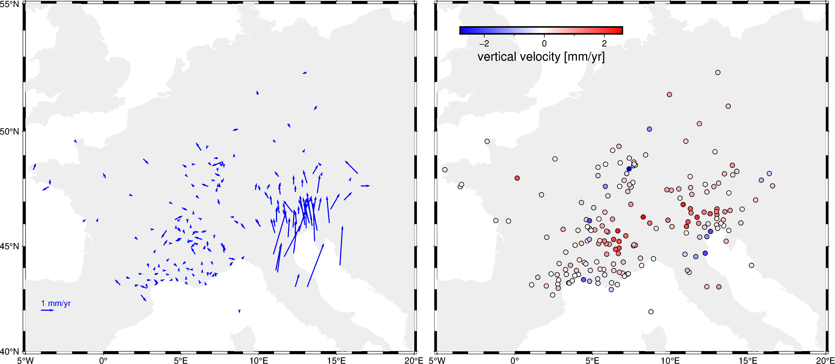
This is a compilation of 3D GPS velocities for the Alps. The horizontal velocities are reference to the Eurasian frame. All velocity components and even the position have error estimates, which is very useful and rare to find in a lot of datasets.
Original source: Sánchez et al. (2018)
import numpy as np
import pandas as pd
import pygmt

import ensaio
Download and cache the data and return the path to it on disk
fname = ensaio.fetch_alps_gps(version=1)
print(fname)
Out:
/home/runner/work/_temp/cache/ensaio/v1/alps-gps-velocity.csv.xz
Load the CSV formatted data with pandas
data = pd.read_csv(fname)
data
To plot the vectors with PyGMT, we need to convert the horizontal components into angle (azimuth) and length.
Now we can make a PyGMT map with the horizontal velocity vectors and vertical velocities encoded as colored points.
# West, East, South, North boundaries of the map
region = [-5, 20, 40, 55]

fig = pygmt.Figure()
with fig.subplot(
    nrows=1,
    ncols=2,
    figsize=("35c", "15c"),
    sharey="l",  # shared y-axis on the left side
    frame="WSrt",
):
    with fig.set_panel(0):
        fig.basemap(region=region, projection="M?", frame="af")
        fig.coast(area_thresh=1e4, land="#eeeeee")
        scale_factor = 2 / length.max()
        fig.plot(
            x=data.longitude,
            y=data.latitude,
            direction=[angle, length * scale_factor],
            style="v0.15c+e",
            color="blue",
            pen="1p,blue",
        )
        # Plot a quiver caption
        fig.plot(
            x=-4,
            y=42,
            direction=[[0], [1 * scale_factor]],
            style="v0.15c+e",
            color="blue",
            pen="1p,blue",
        )
        fig.text(
            x=-4,
            y=42.2,
            text="1 mm/yr",
            justify="BL",
            font="10p,Helvetica,blue",
        )
    with fig.set_panel(1):
        fig.basemap(region=region, projection="M?", frame="af")
        fig.coast(area_thresh=1e4, land="#eeeeee")
        pygmt.makecpt(
            cmap="polar",
            series=[data.velocity_up_mmyr.min(), data.velocity_up_mmyr.max()],
        )
        fig.plot(
            x=data.longitude,
            y=data.latitude,
            color=data.velocity_up_mmyr,
            style="c0.2c",
            cmap=True,
            pen="0.5p,black",
        )
        fig.colorbar(
            frame='af+l"vertical velocity [mm/yr]"',
            position="jTL+w7c/0.3c+h+o1/1",
        )
fig.show()
Out:
<IPython.core.display.Image object>
Total running time of the script: ( 0 minutes 7.129 seconds)