Vector Data

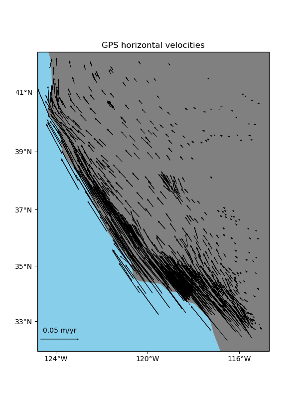
Some datasets have multiple vector components measured for each location, like the East and West components of wind speed or GPS velocities. For example, let’s look at our sample GPS velocity data from the U.S. West coast.

import matplotlib.pyplot as plt
import cartopy.crs as ccrs
import pyproj
import verde as vd

data = vd.datasets.fetch_california_gps()

# We'll need to project the geographic coordinates to work with our Cartesian
# classes/functions
projection = pyproj.Proj(proj="merc", lat_ts=data.latitude.mean())
proj_coords = projection(data.longitude.values, data.latitude.values)
# This will be our desired grid spacing in degrees
spacing = 12 / 60

plt.figure(figsize=(6, 8))
ax = plt.axes(projection=ccrs.Mercator())
crs = ccrs.PlateCarree()
tmp = ax.quiver(
    data.longitude.values,
    data.latitude.values,
    data.velocity_east.values,
    data.velocity_north.values,
    scale=0.3,
    transform=crs,
    width=0.002,
)
ax.quiverkey(tmp, 0.2, 0.15, 0.05, label="0.05 m/yr", coordinates="figure")
ax.set_title("GPS horizontal velocities")
vd.datasets.setup_california_gps_map(ax)
plt.tight_layout()
plt.show()

Out:

/home/leo/src/verde/tutorials/vectors.py:38: UserWarning: Tight layout not applied. The left and right margins cannot be made large enough to accommodate all axes decorations.
  plt.tight_layout()
/home/leo/src/verde/tutorials/vectors.py:39: UserWarning: Matplotlib is currently using agg, which is a non-GUI backend, so cannot show the figure.
  plt.show()

Verde classes and functions are equipped to deal with vector data natively or through the use of the verde.Vector class. Function and classes that can take vector data as input will accept tuples as the data and weights arguments. Each element of the tuple must be an array with the data values for a component of the vector data. As with coordinates, the order of components must be (east_component, north_component, up_component).

Blocked reductions

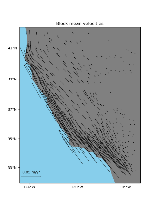
Operations with verde.BlockReduce and verde.BlockMean can handle multi-component data automatically. The reduction operation is applied to each data component separately. The blocked data and weights will be returned in tuples as well following the same ordering as the inputs. This will work for an arbitrary number of components.

# Use a blocked mean with uncertainty type weights
reducer = vd.BlockMean(spacing=spacing * 111e3, uncertainty=True)
block_coords, block_data, block_weights = reducer.filter(
    coordinates=proj_coords,
    data=(data.velocity_east, data.velocity_north),
    weights=(1 / data.std_east ** 2, 1 / data.std_north ** 2),
)
print(len(block_data), len(block_weights))

Out:

2 2

We can convert the blocked coordinates back to longitude and latitude to plot with Cartopy.

block_lon, block_lat = projection(*block_coords, inverse=True)

plt.figure(figsize=(6, 8))
ax = plt.axes(projection=ccrs.Mercator())
crs = ccrs.PlateCarree()
tmp = ax.quiver(
    block_lon,
    block_lat,
    block_data[0],
    block_data[1],
    scale=0.3,
    transform=crs,
    width=0.002,
)
ax.quiverkey(tmp, 0.2, 0.15, 0.05, label="0.05 m/yr", coordinates="figure")
ax.set_title("Block mean velocities")
vd.datasets.setup_california_gps_map(ax)
plt.tight_layout()
plt.show()

Out:

/home/leo/src/verde/tutorials/vectors.py:90: UserWarning: Tight layout not applied. The left and right margins cannot be made large enough to accommodate all axes decorations.
  plt.tight_layout()
/home/leo/src/verde/tutorials/vectors.py:91: UserWarning: Matplotlib is currently using agg, which is a non-GUI backend, so cannot show the figure.
  plt.show()

Trends

Trends can’t handle vector data automatically, so you can’t pass data=(data.velocity_east, data.velocity_north) to verde.Trend.fit. To get around that, you can use the verde.Vector class to create multi-component estimators and gridders from single component ones.

Vector takes an estimator/gridder for each data component and implements the gridder interface for vector data, fitting each estimator/gridder given to a different component of the data.

For example, to fit a trend to our GPS velocities, we need to make a 2-component vector trend:

trend = vd.Vector([vd.Trend(4), vd.Trend(1)])
print(trend)

Out:

Vector(components=[Trend(degree=4), Trend(degree=1)])

We can use the trend as if it were a regular verde.Trend but passing in 2-component data to fit. This will fit each data component to a different verde.Trend.

trend.fit(
    coordinates=proj_coords,
    data=(data.velocity_east, data.velocity_north),
    weights=(1 / data.std_east ** 2, 1 / data.std_north ** 2),
)

Out:

Vector(components=[Trend(degree=4), Trend(degree=1)])

Each estimator can be accessed through the components attribute:

print(trend.components)
print("East trend coefficients:", trend.components[0].coef_)
print("North trend coefficients:", trend.components[1].coef_)

Out:

[Trend(degree=4), Trend(degree=1)]
East trend coefficients: [-3.31743842e+03 -1.61368023e-03 -1.08568612e-03 -2.77735425e-10
 -2.99424188e-10  7.38718817e-12 -2.03916793e-17 -2.68710016e-17
  3.36222190e-18  2.00921241e-18 -5.43959102e-25 -7.79030546e-25
  2.71546631e-25  2.44086928e-25  5.03611061e-26]
North trend coefficients: [-3.35415183e-01 -4.50275691e-08 -3.75590521e-08]

When we call verde.Vector.predict or verde.Vector.grid, we’ll get back predictions for two components instead of just one. Each prediction comes from a different verde.Trend.

pred_east, pred_north = trend.predict(proj_coords)

# Make histograms of the residuals
plt.figure(figsize=(6, 5))
ax = plt.axes()
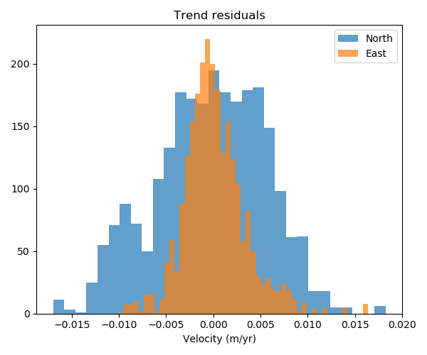
ax.set_title("Trend residuals")
ax.hist(data.velocity_north - pred_north, bins="auto", label="North", alpha=0.7)
ax.hist(data.velocity_east - pred_east, bins="auto", label="East", alpha=0.7)
ax.legend()
ax.set_xlabel("Velocity (m/yr)")
plt.tight_layout()
plt.show()

Out:

/home/leo/src/verde/tutorials/vectors.py:146: UserWarning: Matplotlib is currently using agg, which is a non-GUI backend, so cannot show the figure.
  plt.show()

As expected, the residuals are higher for the North component because of the lower degree polynomial.

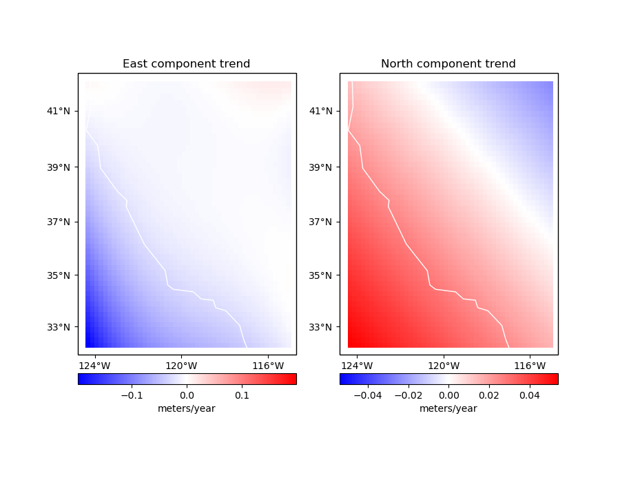
Let’s make geographic grids of these trends.

region = vd.get_region((data.longitude, data.latitude))

grid = trend.grid(
    region=region,
    spacing=spacing,
    projection=projection,
    dims=["latitude", "longitude"],
)
print(grid)

Out:

<xarray.Dataset>
Dimensions:          (latitude: 49, longitude: 47)
Coordinates:
  * longitude        (longitude) float64 235.7 235.9 236.1 ... 244.6 244.8 245.0
  * latitude         (latitude) float64 32.29 32.49 32.69 ... 41.5 41.7 41.9
Data variables:
    east_component   (latitude, longitude) float64 -0.1983 -0.1853 ... 0.01365
    north_component  (latitude, longitude) float64 0.0541 0.05328 ... -0.02427
Attributes:
    metadata:  Generated by Vector(components=[Trend(degree=4), Trend(degree=...

By default, the names of the data components in the xarray.Dataset are east_component and north_component. This can be customized using the data_names argument.

Now we can map the trends.

fig, axes = plt.subplots(
    1, 2, figsize=(9, 7), subplot_kw=dict(projection=ccrs.Mercator())
)
crs = ccrs.PlateCarree()
titles = ["East component trend", "North component trend"]
components = [grid.east_component, grid.north_component]
for ax, component, title in zip(axes, components, titles):
    ax.set_title(title)
    maxabs = vd.maxabs(component)
    tmp = component.plot.pcolormesh(
        ax=ax,
        vmin=-maxabs,
        vmax=maxabs,
        cmap="bwr",
        transform=crs,
        add_colorbar=False,
        add_labels=False,
    )
    cb = plt.colorbar(tmp, ax=ax, orientation="horizontal", pad=0.05)
    cb.set_label("meters/year")
    vd.datasets.setup_california_gps_map(ax, land=None, ocean=None)
    ax.coastlines(color="white")
plt.tight_layout()
plt.show()

Out:

/home/leo/src/verde/tutorials/vectors.py:193: UserWarning: Tight layout not applied. The left and right margins cannot be made large enough to accommodate all axes decorations.
  plt.tight_layout()
/home/leo/src/verde/tutorials/vectors.py:194: UserWarning: Matplotlib is currently using agg, which is a non-GUI backend, so cannot show the figure.
  plt.show()

Gridding

You can use verde.Vector to create multi-component gridders out of verde.Spline the same way as we did for trends. In this case, each component is treated separately.

We can start by splitting the data into training and testing sets (see Model Selection). Notice that verde.train_test_split work for multicomponent data automatically.

train, test = vd.train_test_split(
    coordinates=proj_coords,
    data=(data.velocity_east, data.velocity_north),
    weights=(1 / data.std_east ** 2, 1 / data.std_north ** 2),
    random_state=1,
)

Now we can make a 2-component spline. Since verde.Vector implements fit, predict, and filter, we can use it in a verde.Chain to build a pipeline.

We need to use a bit of damping so that the weights can be taken into account. Splines without damping provide a perfect fit to the data and ignore the weights as a consequence.

chain = vd.Chain(
    [
        ("mean", vd.BlockMean(spacing=spacing * 111e3, uncertainty=True)),
        ("trend", vd.Vector([vd.Trend(1), vd.Trend(1)])),
        ("spline", vd.Vector([vd.Spline(damping=1e-10), vd.Spline(damping=1e-10)])),
    ]
)
print(chain)

Out:

Chain(steps=[('mean',
              BlockMean(adjust='spacing', center_coordinates=False,
                        drop_coords=True, region=None, shape=None,
                        spacing=22200.0, uncertainty=True)),
             ('trend', Vector(components=[Trend(degree=1), Trend(degree=1)])),
             ('spline',
              Vector(components=[Spline(damping=1e-10, engine='auto',
                                        force_coords=None, mindist=1e-05),
                                 Spline(damping=1e-10, engine='auto',
                                        force_coords=None, mindist=1e-05)]))])

Warning

Never generate the component gridders with [vd.Spline()]*2. This will result in each component being a represented by the same Spline object, causing problems when trying to fit it to different components.

Fitting the spline and gridding is exactly the same as what we’ve done before.

chain.fit(*train)

# Score on the test data
print(chain.score(*test))

grid = chain.grid(
    region=region,
    spacing=spacing,
    projection=projection,
    dims=["latitude", "longitude"],
)
print(grid)

Out:

0.9926767145897033
<xarray.Dataset>
Dimensions:          (latitude: 49, longitude: 47)
Coordinates:
  * longitude        (longitude) float64 235.7 235.9 236.1 ... 244.6 244.8 245.0
  * latitude         (latitude) float64 32.29 32.49 32.69 ... 41.5 41.7 41.9
Data variables:
    east_component   (latitude, longitude) float64 -0.04659 ... -0.0006129
    north_component  (latitude, longitude) float64 0.08794 ... -0.0006047
Attributes:
    metadata:  Generated by Chain(steps=[('mean',\n              BlockMean(ad...

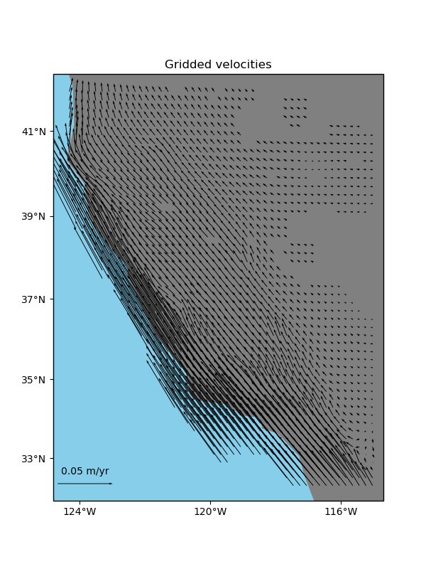
Mask out the points too far from data and plot the gridded vectors.

grid = vd.distance_mask(
    (data.longitude, data.latitude),
    maxdist=spacing * 2 * 111e3,
    grid=grid,
    projection=projection,
)

plt.figure(figsize=(6, 8))
ax = plt.axes(projection=ccrs.Mercator())
tmp = ax.quiver(
    grid.longitude.values,
    grid.latitude.values,
    grid.east_component.values,
    grid.north_component.values,
    scale=0.3,
    transform=crs,
    width=0.002,
)
ax.quiverkey(tmp, 0.2, 0.15, 0.05, label="0.05 m/yr", coordinates="figure")
ax.set_title("Gridded velocities")
vd.datasets.setup_california_gps_map(ax)
plt.tight_layout()
plt.show()

Out:

/home/leo/miniconda3/envs/verde/lib/python3.7/site-packages/cartopy/mpl/geoaxes.py:1752: RuntimeWarning: invalid value encountered in less
  u, v = self.projection.transform_vectors(t, x, y, u, v)
/home/leo/miniconda3/envs/verde/lib/python3.7/site-packages/cartopy/mpl/geoaxes.py:1752: RuntimeWarning: invalid value encountered in greater
  u, v = self.projection.transform_vectors(t, x, y, u, v)
/home/leo/src/verde/tutorials/vectors.py:280: UserWarning: Tight layout not applied. The left and right margins cannot be made large enough to accommodate all axes decorations.
  plt.tight_layout()
/home/leo/src/verde/tutorials/vectors.py:281: UserWarning: Matplotlib is currently using agg, which is a non-GUI backend, so cannot show the figure.
  plt.show()

GPS/GNSS data

For some types of vector data, like GPS/GNSS displacements, the vector components are coupled through elasticity. In these cases, elastic Green’s functions can be used to achieve better interpolation results. The Erizo package implements some of these Green’s functions.

Warning

The verde.VectorSpline2D class implemented an elastically coupled Green’s function but it is deprecated and will be removed in Verde v2.0.0. Please use the implementation in the Erizo package instead.