Note
Click here to download the full example code
Model Selection
The Green’s functions based interpolations in Verde are all linear regressions under the
hood. This means that we can use some of the same tactics from
sklearn.model_selection to evaluate our interpolator’s performance. Once we have
a quantified measure of the quality of a given fitted gridder, we can use it to tune the
gridder’s parameters, like damping for a Spline.
Verde provides adaptations of common scikit-learn tools to work better with spatial
data. Let’s use these tools to evaluate and tune a Spline to grid our
sample air temperature data.
import numpy as np
import matplotlib.pyplot as plt
import cartopy.crs as ccrs
import itertools
import pyproj
import verde as vd

data = vd.datasets.fetch_texas_wind()

# Use Mercator projection because Spline is a Cartesian gridder
projection = pyproj.Proj(proj="merc", lat_ts=data.latitude.mean())
proj_coords = projection(data.longitude.values, data.latitude.values)

region = vd.get_region((data.longitude, data.latitude))
# The desired grid spacing in degrees (converted to meters using 1 degree approx. 111km)
spacing = 15 / 60
Splitting the data
We can’t evaluate a gridder on the data that went into fitting it. The true test of a
model is if it can correctly predict data that it hasn’t seen before. scikit-learn has
the sklearn.model_selection.train_test_split function to separate a dataset
into two parts: one for fitting the model (called training data) and a separate one
for evaluating the model (called testing data). Using it with spatial data would
involve some tedious array conversions so Verde implements
verde.train_test_split which does the same thing but takes coordinates and
data arrays instead.
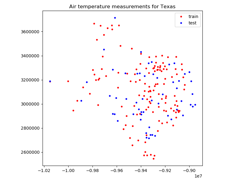
The split is done randomly so we specify a seed for the random number generator to guarantee that we’ll get the same result every time we run this example. You probably don’t want to do that for real data. We’ll keep 30% of the data to use for testing.
train, test = vd.train_test_split(
    proj_coords, data.air_temperature_c, test_size=0.3, random_state=0
)
print(train)
print(test)

plt.figure(figsize=(8, 6))
ax = plt.axes()
ax.set_title("Air temperature measurements for Texas")
ax.plot(train[0][0], train[0][1], ".r", label="train")
ax.plot(test[0][0], test[0][1], ".b", label="test")
ax.legend()
ax.set_aspect("equal")
plt.tight_layout()
plt.show()
Out:
((array([ -9471409.04145469,  -9242651.69892226,  -9518618.69368064,
        -9226352.10603726,  -9196090.97662381,  -9211980.21676049,
        -9111443.79343314,  -9285738.73749109,  -9261270.26198931,
        -9322307.84752338,  -9449918.0091497 ,  -9210462.8659006 ,
        -9437254.33247619,  -9336002.17761117,  -9770852.03064925,
        -9286998.42499748,  -9121969.81858083,  -9225655.46067393,
        -9784479.55912689,  -9724577.60096593,  -9119011.46155829,
        -9366406.45333221,  -9104334.19349208,  -9468488.85678097,
        -9512730.60889723,  -9752004.43349022,  -9474730.03578958,
        -9295711.26358295,  -9407680.30533891,  -9409483.94881389,
        -9113314.23851832,  -9581641.24134595,  -9051780.41245142,
        -9151620.1904154 ,  -9526253.16341599,  -9370920.33356321,
        -9422548.43514848,  -9363887.07831951,  -9926719.2733836 ,
        -9263865.98169933, -10151535.32091524,  -9105488.90703955,
        -9399024.72527645,  -9275584.89274308,  -9287132.02821771,
        -9254036.60191507,  -9356519.81502485,  -9300826.35830558,
        -9088836.21992941,  -9329331.55967991,  -9705882.69320157,
        -9544881.26957023,  -9339151.39637705,  -9260420.92723128,
        -9092882.48888909,  -9202923.82703691,  -9252023.01052236,
        -9250143.02235004,  -9110031.41653215,  -9210586.92603379,
        -9192082.88001273,  -9144987.74483283,  -9265793.68530754,
        -9038200.59940965,  -9241182.06349818,  -9289031.10256449,
        -9405189.55958775,  -9354792.51624734,  -9330810.73819114,
        -9321372.62498082,  -9228556.55917335,  -9199536.03109192,
        -9278581.42211417,  -9229978.47916156,  -9319244.51654206,
        -9297171.35591977,  -9275775.75448643,  -9559682.59776963,
        -9197073.91460223,  -9491697.64477644,  -9185221.40033809,
        -9486172.19730542,  -9098512.91031894,  -9357970.36427463,
        -9348971.2330741 ,  -9415391.11977161,  -9570580.80331692,
        -9298450.12960044,  -9786178.22864295,  -9638164.94664899,
        -9374995.23178449,  -9135062.93417687,  -9363782.10436067,
        -9061161.26713871,  -9641390.51011218,  -9244388.540787  ,
        -9743587.43060695,  -9128583.17798902,  -9688294.78354872,
        -9878049.52882075,  -9261222.54655341,  -9959308.91606633,
        -9374995.23178449,  -9324979.91193078, -10002090.57584577,
        -9291378.70200816,  -9717038.56210237,  -9108943.50459486,
        -9187130.01777196,  -9178474.43770947,  -9821430.39264604,
        -9676089.17505937,  -9590325.45066986,  -9334752.033192  ,
        -9349658.33535029,  -9217667.89671333,  -9192989.47329381,
        -9735189.51389807,  -9062249.17907602,  -9332852.95884533,
        -9455815.63702027,  -9796236.64251932,  -9443505.05457202,
        -9320723.69505337,  -9754266.14514927,  -9765097.54908629,
        -9081077.6900608 ,  -9042075.09280036,  -9433427.55452137,
        -9587615.21391383]), array([2657710.28293861, 3302077.73567252, 2899046.15133399,
       2838589.68737716, 3049850.71722841, 3290767.45780106,
       2931160.45084784, 3271137.71227972, 3285325.92731206,
       3104893.52310543, 3247812.59589509, 3166662.55342553,
       3287606.04132201, 3103141.68482877, 3197876.76156001,
       3149242.24908431, 3067381.83156894, 3400585.90023853,
       3243911.5995015 , 3290869.09139339, 2992634.70248073,
       3169418.17605082, 3246497.10552017, 2817264.46474637,
       3252930.02674656, 3200327.43647367, 3459184.29516942,
       3112292.18628403, 2917869.77563751, 3197809.62807528,
       3290225.42947942, 3652939.53050434, 3222645.66433888,
       2963817.97546003, 2824339.57488837, 3107155.82534808,
       2698337.04679593, 2601703.23660133, 3025820.22660258,
       3166283.29483646, 3185632.21052805, 3023883.40574366,
       3417009.35720713, 3393428.62105992, 3316162.95136998,
       3082031.84084665, 2953318.41751121, 2933549.90421567,
       2932676.98398158, 3020406.81467849, 3574040.01091358,
       2790505.48355738, 2973418.65910265, 3307698.11129963,
       2945505.02203083, 3311522.23776725, 2975313.52946633,
       2861050.32840049, 2887880.3960125 , 2945898.28967202,
       2941474.84700705, 3225124.76062141, 3281387.74953726,
       3159592.7976058 , 3315823.31326006, 2571845.86314015,
       3331844.27865595, 2740231.34771917, 3387759.04557859,
       3060081.02436476, 3041845.53079301, 3210124.8374159 ,
       3164074.94938398, 3271836.50108902, 2579123.45324659,
       2545954.59014788, 3342747.49976745, 2979356.30060547,
       3009203.6131726 , 2719110.10495866, 2846814.97160994,
       3188985.42191104, 2983466.36042869, 3294675.45126596,
       3039773.54716658, 3071437.56540843, 3483134.04990316,
       3294607.6695262 , 3667917.1194501 , 3619924.68699415,
       2573548.51452294, 2821249.74463368, 2683074.91768678,
       3285461.36507139, 3652271.03785312, 3283204.30900926,
       3210853.02111693, 2943844.71518428, 3230601.11578242,
       3137567.17555595, 2777047.34270749, 2945144.53916802,
       3066497.95513723, 3110760.99744545, 3188091.12461516,
       3298991.83921469, 3394820.85278175, 3391739.95155904,
       3286590.08456857, 3389059.21988513, 3085628.36101872,
       3630202.83368938, 3134419.72201147, 3256654.45390054,
       2573738.88783378, 3339785.07776942, 3063935.13249589,
       3648601.05705207, 3330211.5352512 , 3142162.17467495,
       2982622.30031315, 3282673.97488324, 3183676.67838886,
       3006522.74236789, 2990221.2234946 , 3532083.29147308,
       2942206.50247381, 3121339.67312345, 2913261.59698676,
       3259243.23756798])), (array([18.15166667, 12.17857143, 16.45916667, 16.60084507, 12.41170213,
        9.67159091, 16.33043478,  9.43978723, 11.10313725, 10.22955556,
       11.57575758, 12.47194444, 12.22138889, 10.36794118,  8.775     ,
       10.46055556, 12.55241379, 11.78611111,  7.89736111,  7.06944444,
       14.57882353, 12.33319444, 11.96138889, 16.88692308, 10.20833333,
        9.1525    ,  9.64888889, 10.29677419, 15.16444444, 12.81565217,
       10.        ,  3.16277778, 13.49071429, 14.98529412, 16.66666667,
       13.06835821, 16.63416667, 20.43375   ,  5.96285714, 13.76470588,
        9.16391304, 13.8736    , 10.99888889, 11.23633803,  9.751875  ,
       12.43888889, 10.94418605, 15.23805556, 16.66589744, 11.40892857,
        4.984     , 18.08955224, 11.45891304, 12.05545455, 16.13939394,
       11.18275362, 14.49676056, 15.90777778, 18.8625    , 14.27527778,
       14.97291667, 10.73239437,  8.98125   , 11.89032258, 11.46025641,
       22.6082    , 10.77111111, 16.40823529,  9.23611111, 10.82863636,
       12.57958333, 11.18545455, 11.13193548, 10.56277778, 20.97333333,
       23.26113208, 10.365     , 14.46875   , 14.21430556, 16.8525    ,
       17.01530612, 12.83722222, 15.22228571,  9.005     , 14.1       ,
       14.19444444,  9.02333333, 12.11923077,  2.1525    ,  5.64638889,
       21.09483871, 19.73611111, 18.09676056, 11.48449275,  4.29166667,
        9.78117647, 10.1875    , 16.36536585,  8.73277778,  7.70694444,
       17.2974    , 15.35777778, 14.53130435, 16.58333333,  7.52666667,
       11.37028571,  5.79375   ,  8.54088235,  9.196     , 10.37263889,
       11.39375   ,  7.08166667, 11.74291667, 10.86027778, 20.47454545,
       10.9936    , 12.47652778,  3.43633803, 10.0825    ,  9.59677419,
       13.55277778,  6.09319444, 20.58333333, 11.65820513, 14.4926087 ,
        3.14875   , 16.80952381, 12.45724138, 15.76208333, 11.69902778]),), (None,))
((array([ -9355174.23973406,  -9305731.50511056,  -9378946.06987249,
        -9894654.50049513,  -9357159.20186525,  -9310436.24708494,
        -9176098.20900436,  -9848465.95859632,  -9657890.50782771,
        -9408987.70828107,  -9592090.92179619,  -9397058.84931958,
        -9614660.3229513 ,  -9438991.174341  ,  -9220530.82286406,
        -9464280.35533937,  -9148327.82534205,  -9254885.93667311,
        -9284574.48085645,  -9103675.72047743,  -9617332.38735867,
        -9038401.00424027,  -9631570.67341502,  -9133335.63539924,
        -9125099.95117223,  -9369183.49169843,  -8985427.32736408,
        -9520794.51755526,  -9397182.90945276,  -8972410.55646536,
        -9418511.70927591,  -9312192.17512407,  -9633794.21272551,
        -9386466.02256181,  -9298192.46624686, -10151936.13057628,
        -9335849.48821648,  -9334064.93091582,  -8951759.31583123,
        -9066696.25769684,  -9086927.60249552,  -9399253.75936852,
        -9167595.31833663,  -9052610.66103518,  -9401849.47907855,
        -9332280.37361521,  -8991029.11953241,  -8973832.47645353,
        -9529249.69278712,  -9266070.43483542,  -9429505.34569483,
        -8999875.56133822,  -9322689.57101016,  -9604983.63256177,
        -9104467.79671247,  -9706970.60513881]), array([2719870.27460582, 2743685.56324252, 2933768.14517002,
       3027361.13101297, 2757426.84021469, 3028296.78889616,
       2903724.5557224 , 3182157.20869187, 3066100.23492454,
       3255225.28091213, 2860584.19616269, 2934171.90242785,
       3714012.76916745, 3011874.16439619, 3080991.84629854,
       2915167.81938923, 2873187.46869299, 3003831.55941359,
       2735051.95799933, 2953788.49303643, 2915178.71303919,
       3249859.25595487, 2916780.19714376, 3182123.69352164,
       3337515.62533228, 3230904.19741824, 3187923.45258656,
       3041327.49695636, 2912727.91396922, 2979696.00616845,
       2954947.37073634, 3348209.3192316 , 3284716.48014213,
       3043124.19066597, 3246452.13452785, 3189924.51834186,
       3339251.70946121, 2715192.27113021, 2992766.36237038,
       3024323.56139652, 3192216.72345509, 3430837.16378734,
       3327060.19688609, 2904921.67586422, 2871114.86619099,
       2807032.29570529, 2992876.08017689, 3082728.91614068,
       3254021.33225593, 3216131.11265389, 3253177.52895142,
       3265222.50231349, 2744264.94274218, 3049585.98626738,
       3129450.2499978 , 3452568.99011507])), (array([17.71611111, 17.3918    , 10.73421875,  8.08555556, 16.258125  ,
       16.18181818, 15.87828571,  7.47625   , 11.02857143, 12.25472222,
       17.16923077, 15.60208333,  5.04152778, 13.14263889, 12.47835821,
       16.69304348, 18.73916667, 11.46194444, 18.38255319, 16.02173913,
       16.57884615, 10.55866667, 16.48916667, 13.43583333, 10.67041667,
       11.90319444, 11.49557143, 12.17826087, 14.27805556, 17.43382353,
       12.95833333, 11.04708333,  9.60486111, 13.46      , 10.58730159,
        7.39333333, 10.11722222, 17.7375    , 17.10013889, 14.64180556,
       12.44957143,  9.68391304, 11.93055556, 20.34757576, 15.4025    ,
       16.76319444, 17.33347222, 13.55152778, 10.49541667, 11.92041667,
       10.42583333, 12.69078125, 17.22138889, 10.33333333, 12.80555556,
        3.85638889]),), (None,))
The returned train and test arguments are each tuples with the coordinates (in
a tuple) and a data array. They are in a format that can be easily passed to the
fit method of most gridders using Python’s argument
expansion using the * symbol.
chain = vd.Chain(
    [
        ("reduce", vd.BlockReduce(np.mean, spacing * 111e3)),
        ("trend", vd.Trend(degree=1)),
        ("spline", vd.Spline()),
    ]
)
chain.fit(*train)
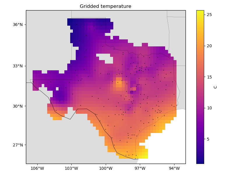
Let’s plot the gridded result to see what it looks like. We’ll mask out grid points that are too far from any given data point.
mask = vd.distance_mask(
    (data.longitude, data.latitude),
    maxdist=3 * spacing * 111e3,
    coordinates=vd.grid_coordinates(region, spacing=spacing),
    projection=projection,
)
grid = chain.grid(
    region=region,
    spacing=spacing,
    projection=projection,
    dims=["latitude", "longitude"],
    data_names=["temperature"],
).where(mask)

plt.figure(figsize=(8, 6))
ax = plt.axes(projection=ccrs.Mercator())
ax.set_title("Gridded temperature")
pc = ax.pcolormesh(
    grid.longitude,
    grid.latitude,
    grid.temperature,
    cmap="plasma",
    transform=ccrs.PlateCarree(),
)
plt.colorbar(pc).set_label("C")
ax.plot(data.longitude, data.latitude, ".k", markersize=1, transform=ccrs.PlateCarree())
vd.datasets.setup_texas_wind_map(ax)
plt.tight_layout()
plt.show()
Scoring
Gridders in Verde implement the score method that
calculates the R² coefficient of determination
for a given comparison dataset (test in our case). The R² score is at most 1,
meaning a perfect prediction, but has no lower bound.
score = chain.score(*test)
print("R² score:", score)
Out:
R² score: 0.8455402431159149
That’s a good score meaning that our gridder is able to accurately predict data that wasn’t used in the gridding algorithm.
Tuning
Spline has many parameters that can be set to modify the final result.
Mainly the damping regularization parameter and the mindist “fudge factor”
which smooths the solution. Would changing the default values give us a better score?
What if we used a 2nd degree trend instead?
We can answer these questions by changing the values in our chain and
re-evaluating the model score. Let’s test the following combinations of parameters:
dampings = [None, 1e-8, 1e-6]
mindists = [10e3, 100e3, 1000e3]
degrees = [1, 2, 3, 4]

# Use itertools to create a list with all combinations of parameters to test
parameter_sets = list(itertools.product(dampings, mindists, degrees))
print("Number of combinations:", len(parameter_sets))
print("Combinations:", parameter_sets)
Out:
Number of combinations: 36
Combinations: [(None, 10000.0, 1), (None, 10000.0, 2), (None, 10000.0, 3), (None, 10000.0, 4), (None, 100000.0, 1), (None, 100000.0, 2), (None, 100000.0, 3), (None, 100000.0, 4), (None, 1000000.0, 1), (None, 1000000.0, 2), (None, 1000000.0, 3), (None, 1000000.0, 4), (1e-08, 10000.0, 1), (1e-08, 10000.0, 2), (1e-08, 10000.0, 3), (1e-08, 10000.0, 4), (1e-08, 100000.0, 1), (1e-08, 100000.0, 2), (1e-08, 100000.0, 3), (1e-08, 100000.0, 4), (1e-08, 1000000.0, 1), (1e-08, 1000000.0, 2), (1e-08, 1000000.0, 3), (1e-08, 1000000.0, 4), (1e-06, 10000.0, 1), (1e-06, 10000.0, 2), (1e-06, 10000.0, 3), (1e-06, 10000.0, 4), (1e-06, 100000.0, 1), (1e-06, 100000.0, 2), (1e-06, 100000.0, 3), (1e-06, 100000.0, 4), (1e-06, 1000000.0, 1), (1e-06, 1000000.0, 2), (1e-06, 1000000.0, 3), (1e-06, 1000000.0, 4)]
Now we can loop over the combinations and collect the scores for each parameter set.
scores = []
for damping, mindist, degree in parameter_sets:
    chain.named_steps["spline"].set_params(damping=damping, mindist=mindist)
    chain.named_steps["trend"].set_params(degree=degree)
    score = chain.fit(*train).score(*test)
    scores.append(score)
print(scores)
Out:
[0.7238830882947062, 0.7070997586193799, 0.7116974741128288, 0.8355207134557427, 0.8625010250415266, 0.8595635581413738, 0.8684356255592811, 0.7631365452241242, 0.8615410794928423, 0.8586131408040516, 0.8673084289960357, 0.7607537665584987, 0.7373990722551209, 0.7232205306525006, 0.727299665943367, 0.8314180120026677, 0.862501007777039, 0.8595634396278273, 0.8684355655474266, 0.7631370161800535, 0.8615410770291272, 0.8586131345908206, 0.8673084255284418, 0.76075378587685, 0.827682619687416, 0.8292355572539247, 0.8305543665058613, 0.7111394283333616, 0.8624996340091982, 0.8595521447764479, 0.8684300027698172, 0.763183252203994, 0.8615408365168034, 0.8586125231165259, 0.8673080855615971, 0.7607556992123854]
The largest score will yield the best parameter combination.
best = np.argmax(scores)
print("Best score:", scores[best])
print("Best damping, mindist, and degree:", parameter_sets[best])
Out:
Best score: 0.8684356255592811
Best damping, mindist, and degree: (None, 100000.0, 3)
We managed to get a slightly better score using the above configuration. That’s not a huge improvement but we also haven’t tried that many parameter combinations.
We can now configure our chain with the best configuration and re-fit. We could also have kept separate chains, each fit on a combination, to avoid having to fit again. Since this is a small dataset, it doesn’t matter too much.
damping, mindist, degree = parameter_sets[best]
chain.named_steps["spline"].set_params(damping=damping, mindist=mindist)
chain.named_steps["trend"].set_params(degree=degree)
chain.fit(*train)
Finally, we can make a grid with the best configuration to see how it compares to our previous result.
grid_best = chain.grid(
    region=region,
    spacing=spacing,
    projection=projection,
    dims=["latitude", "longitude"],
    data_names=["temperature"],
).where(mask)

plt.figure(figsize=(14, 8))
for i, title, grd in zip(range(2), ["Defaults", "Tuned"], [grid, grid_best]):
    ax = plt.subplot(1, 2, i + 1, projection=ccrs.Mercator())
    ax.set_title(title)
    pc = ax.pcolormesh(
        grd.longitude,
        grd.latitude,
        grd.temperature,
        cmap="plasma",
        transform=ccrs.PlateCarree(),
        vmin=data.air_temperature_c.min(),
        vmax=data.air_temperature_c.max(),
    )
    plt.colorbar(pc, orientation="horizontal", aspect=50, pad=0.05).set_label("C")
    ax.plot(
        data.longitude, data.latitude, ".k", markersize=1, transform=ccrs.PlateCarree()
    )
    vd.datasets.setup_texas_wind_map(ax)
plt.tight_layout()
plt.show()
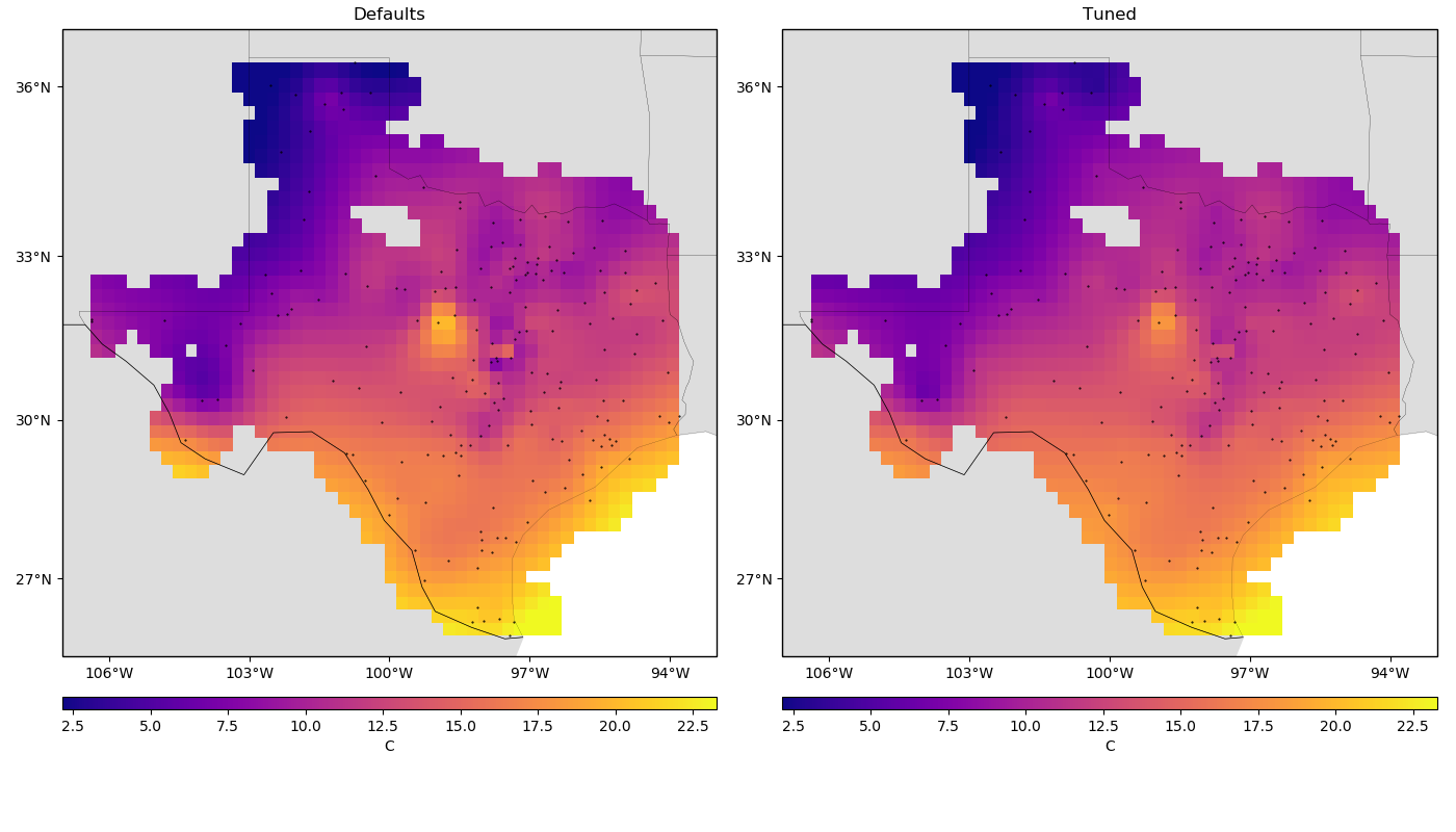
Notice that, for sparse data like these, smoother models tend to be better predictors. This is a sign that you should probably not trust many of the short wavelength features that we get from the defaults.
Total running time of the script: ( 0 minutes 22.207 seconds)