Note
Click here to download the full example code
Data Decimation
Often times, raw spatial data can be highly oversampled in a direction. In these cases, we need to decimate the data before interpolation to avoid aliasing effects.
import matplotlib.pyplot as plt
import cartopy.crs as ccrs
import verde as vd
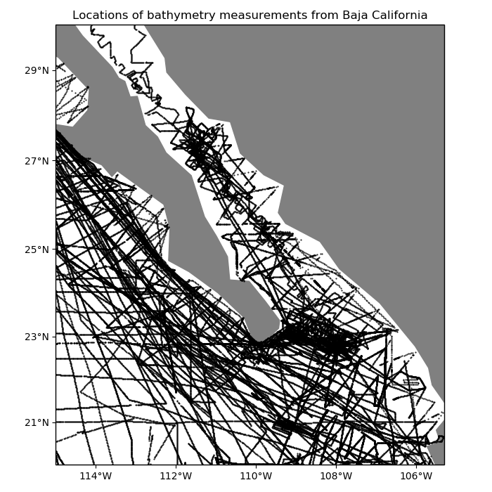
For example, our sample shipborne bathymetry data has a higher sampling frequency along the tracks than between tracks:
# Load the data as a pandas.DataFrame
data = vd.datasets.fetch_baja_bathymetry()

# Plot it using matplotlib and Cartopy
crs = ccrs.PlateCarree()
plt.figure(figsize=(7, 7))
ax = plt.axes(projection=ccrs.Mercator())
ax.set_title("Locations of bathymetry measurements from Baja California")
# Plot the bathymetry data locations as black dots
plt.plot(data.longitude, data.latitude, ".k", markersize=1, transform=crs)
vd.datasets.setup_baja_bathymetry_map(ax)
plt.tight_layout()
plt.show()
Class verde.BlockReduce can be used to apply a reduction/aggregation
operation (mean, median, standard deviation, etc) to the data in regular blocks. All
data inside each block will be replaced by their aggregated value.
BlockReduce takes an aggregation function as input. It can be any
function that receives a numpy array as input and returns a single scalar value. The
numpy.mean or numpy.median functions are usually what we want.
import numpy as np
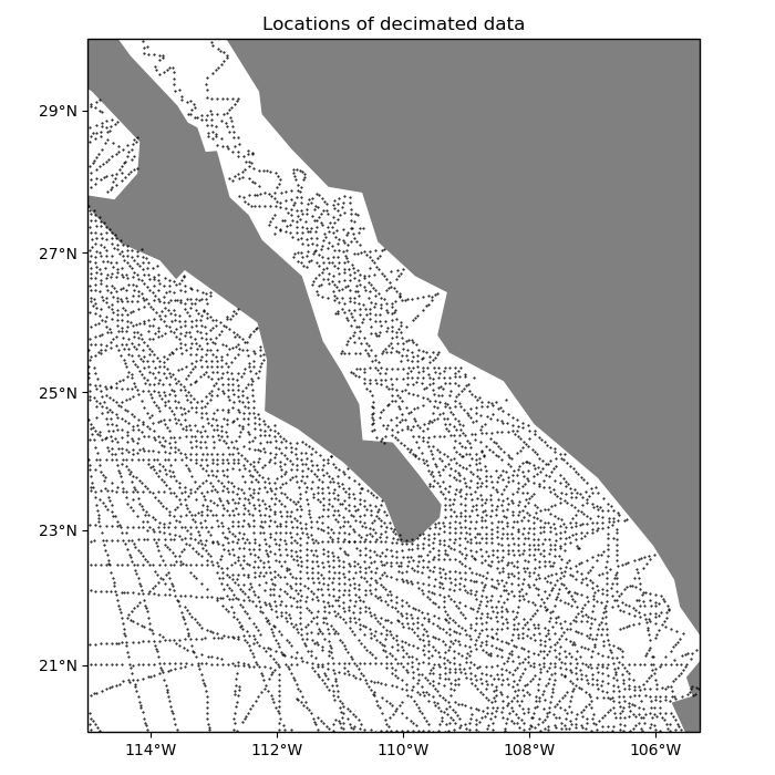
Blocked means and medians are good ways to decimate data for interpolation. Let’s use a blocked median on our data to decimate it to our desired grid interval of 5 arc-minutes. The reason for using a median over a mean is because bathymetry data can vary abruptly and a mean would smooth the data too much. For data varies more smoothly (like gravity and magnetic data), a mean would be a better option.
reducer = vd.BlockReduce(reduction=np.median, spacing=5 / 60)
print(reducer)
Out:
BlockReduce(adjust='spacing', center_coordinates=False,
      reduction=<function median at 0x2ac02e67e510>, region=None,
      spacing=0.08333333333333333)
Use the filter method to apply the reduction:
coordinates, bathymetry = reducer.filter(
    coordinates=(data.longitude, data.latitude), data=data.bathymetry_m
)

plt.figure(figsize=(7, 7))
ax = plt.axes(projection=ccrs.Mercator())
ax.set_title("Locations of decimated data")
# Plot the bathymetry data locations as black dots
plt.plot(*coordinates, ".k", markersize=1, transform=crs)
vd.datasets.setup_baja_bathymetry_map(ax)
plt.tight_layout()
plt.show()
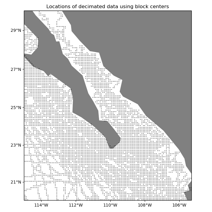
By default, the coordinates of the decimated data are obtained by applying the same
reduction operation to the coordinates of the original data. Alternatively, we can
tell BlockReduce to return the coordinates of the center of each
block:
reducer_center = vd.BlockReduce(
    reduction=np.median, spacing=5 / 60, center_coordinates=True
)
coordinates_center, bathymetry = reducer_center.filter(
    coordinates=(data.longitude, data.latitude), data=data.bathymetry_m
)

plt.figure(figsize=(7, 7))
ax = plt.axes(projection=ccrs.Mercator())
ax.set_title("Locations of decimated data using block centers")
# Plot the bathymetry data locations as black dots
plt.plot(*coordinates_center, ".k", markersize=1, transform=crs)
vd.datasets.setup_baja_bathymetry_map(ax)
plt.tight_layout()
plt.show()
Now the data are ready for interpolation.
Total running time of the script: ( 0 minutes 2.433 seconds)