Detecting Magnetic Sources#

This tutorial demonstrates how to detect magnetic sources in a simulated magnetic field using the total gradient amplitude (TGA) and a Laplacian of Gaussian segmentation algorithm.

Magnetic data#

First, we need magnetic microscopy data to process and apply the detection algorithm. To achieve this, we will use the complex synthetic model.

import numpy as np
import verde as vd
import magali as mg
import harmonica as hm

sensor_sample_distance = 5.0  # µm
region = [0, 2000, 0, 2000]  # µm
spacing = 2  # µm

true_inclination = 30  # degrees
true_declination = 40  # degrees
true_dispersion_angle = 5  # degrees
size = 100  # number of random dipoles

directions_inclination, directions_declination = mg.random_directions(
    true_inclination,
    true_declination,
    true_dispersion_angle,
    size=size,
    random_state=5,
)

dipoles_amplitude = abs(np.random.normal(0, 100, size)) * 1.0e-14

dipole_coordinates = (
    np.concatenate([np.random.randint(30, 1970, size), [1250, 1300, 500]]),  # x
    np.concatenate([np.random.randint(30, 1970, size), [500, 1750, 1000]]),  # y
    np.concatenate([np.random.randint(-20, -1, size), [-15, -15, -30]]),     # z
)

dipole_moments = hm.magnetic_angles_to_vec(
    inclination=np.concatenate([directions_inclination, [10, -10, -5]]),
    declination=np.concatenate([directions_declination, [10, 170, 190]]),
    intensity=np.concatenate([dipoles_amplitude, [5e-11, 5e-11, 5e-11]]),
)

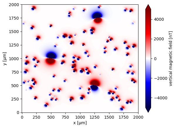
data = mg.dipole_bz_grid(
    region, spacing, sensor_sample_distance,
    dipole_coordinates, dipole_moments
)

data.plot.pcolormesh(cmap="seismic", vmin=-5000, vmax=5000)

<matplotlib.collections.QuadMesh at 0x7fc5d487a2a0>

Source Detection#

The source detection process involves a few signal enhancement and segmentation steps:

Upward continuation: high-frequency noise is reduced.
Total Gradient Amplitude (TGA): signal near magnetic sources is enhanced.
Contrast stretching: weaker signals are highlighted through rescaling.
Laplacian of Gaussian (LoG) segmentation: anomalies are identified by detecting “blobs”.
Ranking: windows are ranked by signal strength to prioritize processing.

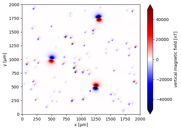
Upward Continuation#

Upward continuation suppresses small-scale noise while preserving larger magnetic anomalies. Using Harmonica, a minimal upward continuation height is applied to retain most of the original signal.

height_difference = 5
data_up = (
    hm.upward_continuation(data, height_difference)
    .assign_attrs(data.attrs)
    .assign_coords(x=data.x, y=data.y)
    .assign_coords(z=data.z + height_difference)
)
data_up.plot.pcolormesh(cmap="seismic", vmin=-50000, vmax=50000)

<matplotlib.collections.QuadMesh at 0x7fc5d4706c90>

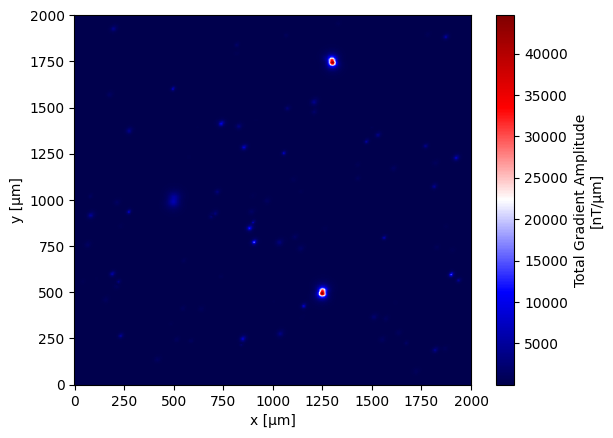
Total Gradient Amplitude (TGA)#

The TGA acts as a high-pass filter, emphasizing regions near magnetic sources.

data_tga = mg.total_gradient_amplitude_grid(data_up)
data_tga.plot.pcolormesh(cmap="seismic")

<matplotlib.collections.QuadMesh at 0x7fc5d4636c90>

Contrast Stretching#

Using skimage, contrast stretching is applied after the TGA calculation to enhance both low and high signal intensities by rescaling the data between its 1st and 99th percentiles.

import skimage.exposure

data_stretched = skimage.exposure.rescale_intensity(
    data_tga,
    in_range=tuple(np.percentile(data_tga, (1, 99))),
)
data_stretched.plot.pcolormesh(cmap="seismic")

<matplotlib.collections.QuadMesh at 0x7fc5d3086c90>

Laplacian of Gaussian (LoG) Segmentation#

The Laplacian of Gaussian (LoG) is a blob detection technique commonly used in image analysis. It identifies regions that differ significantly in intensity compared to their surroundings — often corresponding to compact sources or anomalies. In our case, this is used to detect windows that contain magnetic anomalies, helping to identify potential magnetic grains. The objective is to isolate a single magnetic source within each window

windows = mg.detect_anomalies(
    data_stretched,
    size_range=[25, 50],  # Expected size range of anomalies (µm)
    size_multiplier=2,
    num_scales=10,
    detection_threshold=0.01,
    overlap_ratio=0.5,
    border_exclusion=1,
)

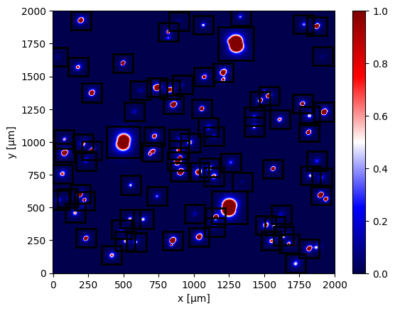
Finally, the data is plotted along with the windows to visually inspect the final results.

import matplotlib
import matplotlib.pyplot as plt

ax = plt.subplot(111)
data_stretched.plot.pcolormesh(ax=ax, cmap="seismic")
for window in windows:
    rect = matplotlib.patches.Rectangle(
        xy=[window[0], window[2]],
        width=window[1] - window[0],
        height=window[3] - window[2],
        edgecolor="k",
        fill=False,
        linewidth=2,
    )
    ax.add_patch(rect)

Detecting Magnetic Sources

Contents